Docs Menu
Tracking and Profile Validation
Import your own CSV observations, review their quality, and save a validation report for an immutable profile snapshot.
Create a CSV source
- Select your Project in Engineering Studies. Open Project Modelling → Profiles → Tracking.
- Under Add a source, enter Source name. Select CSV upload as the connector.
- Confirm that you have permission to import the data. Select Create source.
- Choose CSV file for that source, then select Upload CSV.
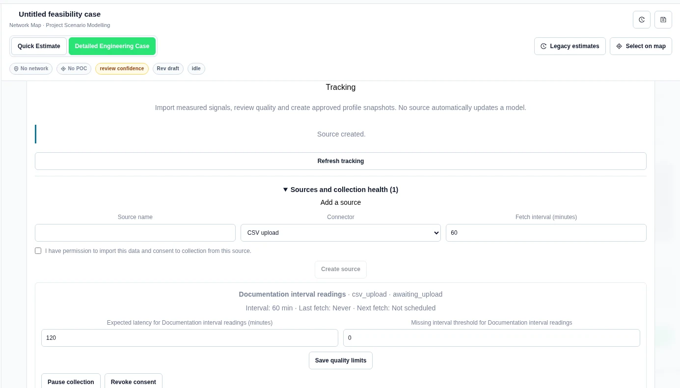
The maximum file size is 2 MB. Use signal,timestamp,value,unit,kind,intervalMinutes. Timestamps need an explicit UTC offset or Z. Supported kinds are energy, power and cashflow. Empty values remain missing. State the correct unit; never infer a currency from a bare number.
Review and approve a snapshot
- In Signal catalogue, select Inspect signal.
- Review the range, cadence, point count, units, missing intervals, null values and observation reasons. Old data can be marked stale even when its supplied rows are complete.
- Under Review profile mapping, enter Profile name and select Profile use.
- If needed, enter explicit Excluded windows with a reason. Review the observations and select the confirmation checkbox.
- Select Approve new profile snapshot.
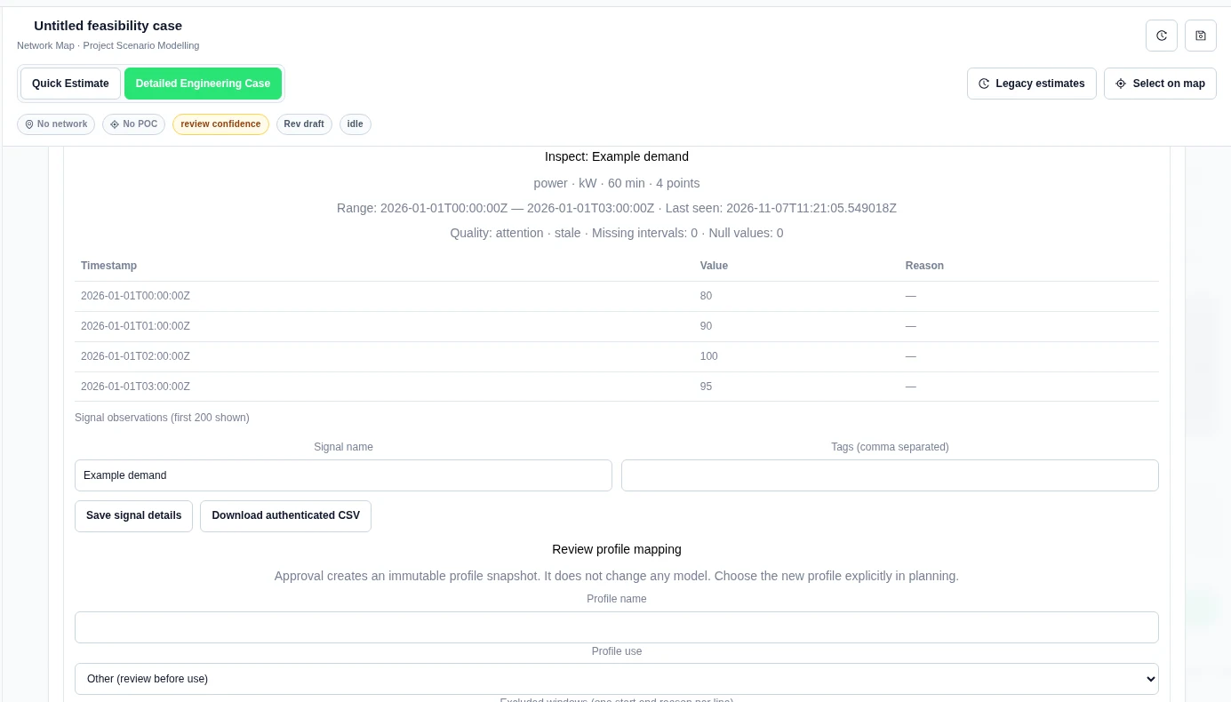
Approval does not replace an input in a model or rerun a case. A later source change does not alter this snapshot. Refresh to new snapshot creates another copy after a new review.
Validate and download
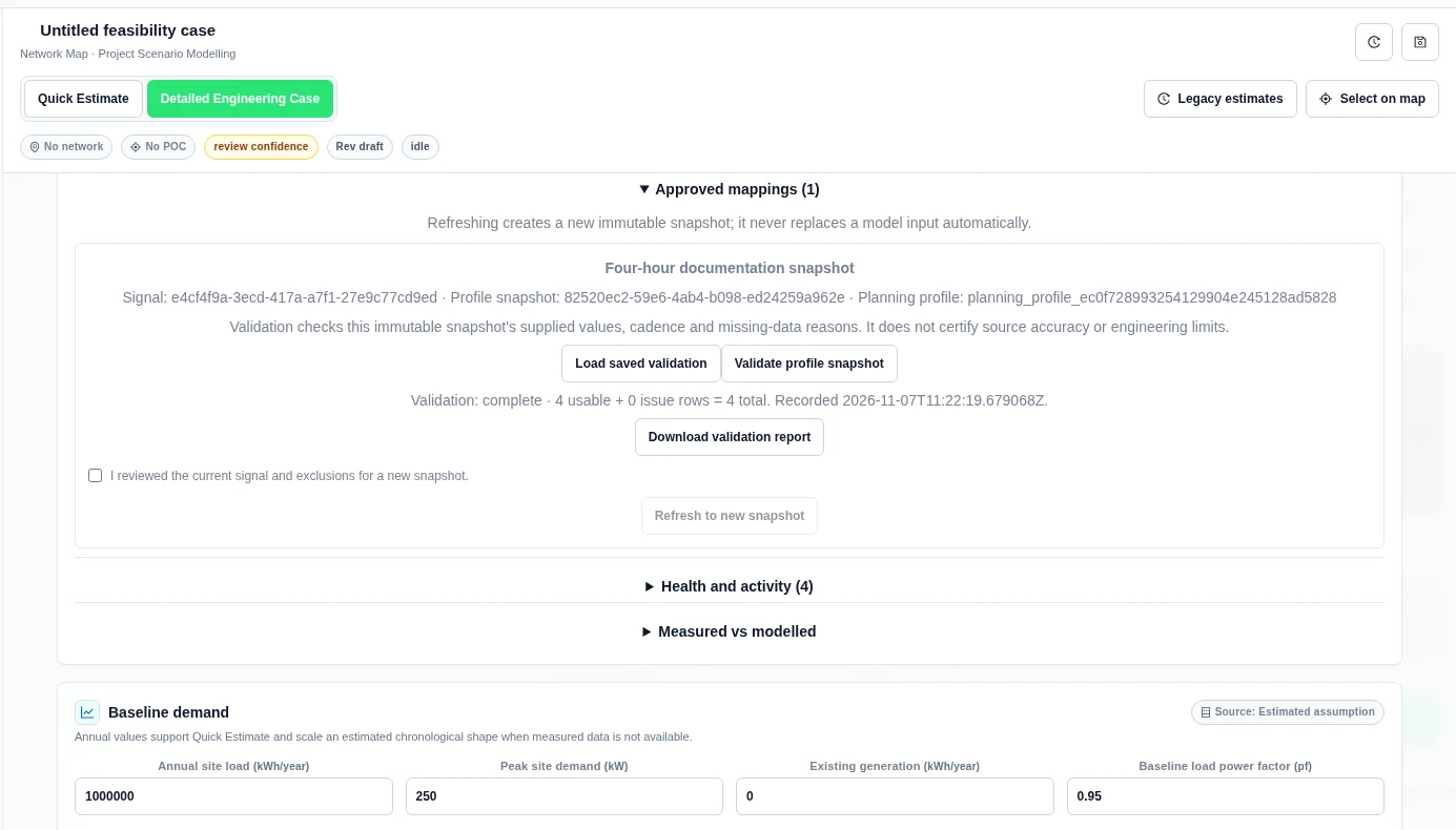
- Expand Approved mappings.
- Select Validate profile snapshot for the intended snapshot.
- Check the reported usable, issue and total row counts.
- Select Download validation report. Keep the JSON report with your input evidence. Load saved validation retrieves the stored outcome later.
Worked example: four hourly observations
We uploaded four example power readings on 1 January 2026 at 00:00, 01:00, 02:00 and 03:00 UTC. The values were 80, 90, 100 and 95 kW, with a 60-minute interval. These were authored demonstration inputs.
The signal displayed 4 points, 0 missing intervals and 0 null values. The saved report returned complete · 4 usable + 0 issue rows = 4 total. It was recorded at 2026-11-07T11:22:19.679068Z. Power values are not added to make an energy total.
Compare a signal with a saved Detailed run
- In Profiles, open Saved Detailed run performance.
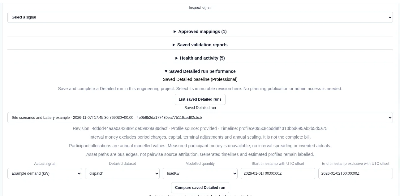
- Under Saved Detailed baseline (Professional), select List saved Detailed runs, then choose a Saved Detailed run.
- Choose the Actual signal, the Detailed dataset (dispatch, asset_paths or money) and the Modelled quantity.
- Enter Start timestamp with UTC offset and End timestamp exclusive with UTC offset.
- Select Compare saved Detailed run.
Worked example: four readings against a full day
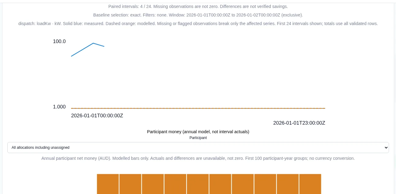
We compared the four-reading Example demand (kW) signal with run 4e05652da177430ea775116ced82c5cb from the North depot example. We chose dispatch and loadKw for 2026-01-01T00:00:00Z to 2026-01-02T00:00:00Z. The result said Paired intervals: 4 / 24. The modelled load was 1 kW in each hour, so the 80–100 kW readings were far above it. The example readings belong to a different scale of site, and the comparison shows that clearly.
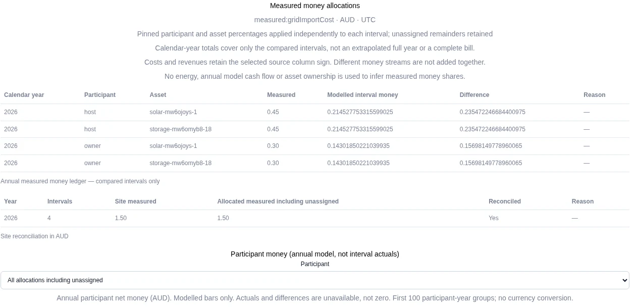
The panel also shows Participant money (annual model, not interval actuals). These are annual modelled values in AUD. The actual and difference columns say "Unavailable — no annual measured allocation".
Limits
- The quality state and snapshot validation answer different questions. Freshness is not the same as completeness within a supplied window.
- Missing or flagged observations are not replaced with zero.
- Validation reports data-quality findings and leaves the snapshot unchanged.
- This guide covers CSV intake, snapshot validation and comparison with saved Detailed runs. Configure external data credentials separately where required.
Allocate measured money by participant and asset
Use a cashflow signal with an explicit currency. This ledger groups the compared intervals by calendar year. It does not turn a short window into a full-year bill.
- In Value, enter participant shares for the required measured: stream. These are separate from ordinary revenue, capital and energy shares.
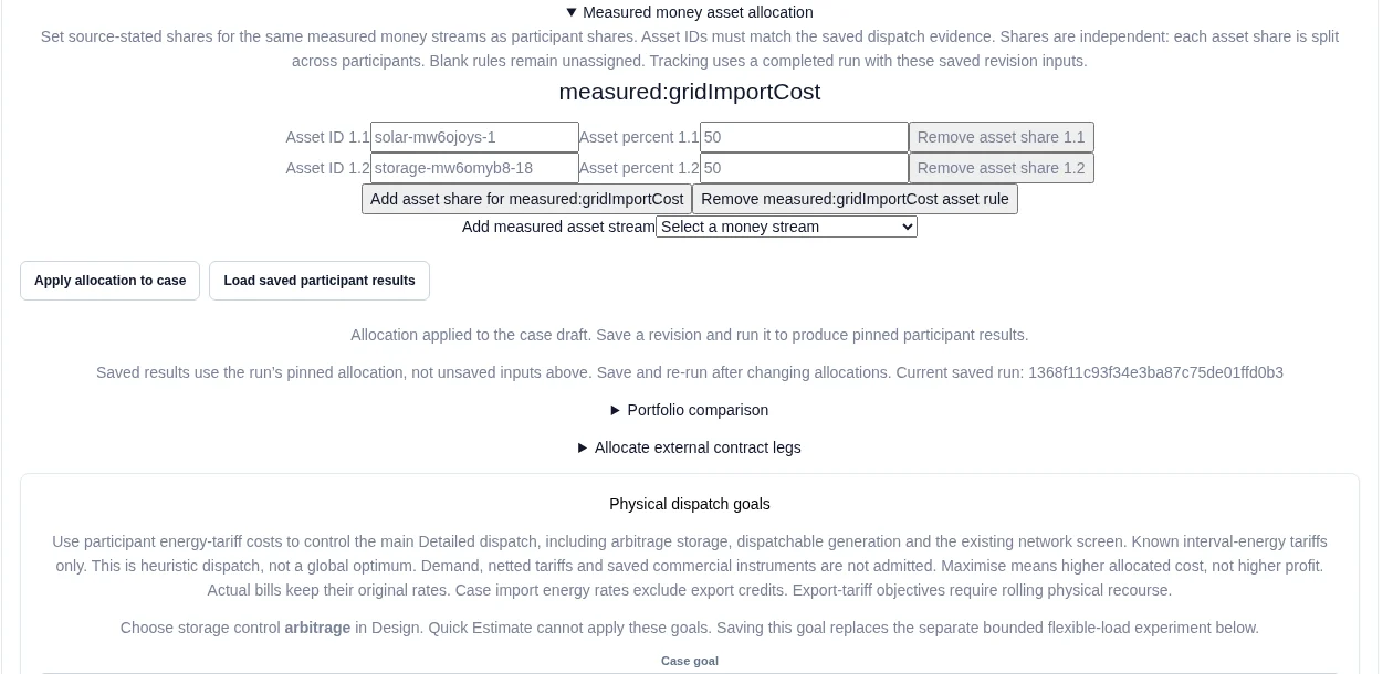
- Expand Measured money asset allocation. Select Add measured asset stream, add asset shares, and use the exact asset IDs from the saved dispatch evidence.
- Select Apply allocation to case. Save a revision and complete a new Detailed run. Later draft edits do not change that run.
Compare the money signal
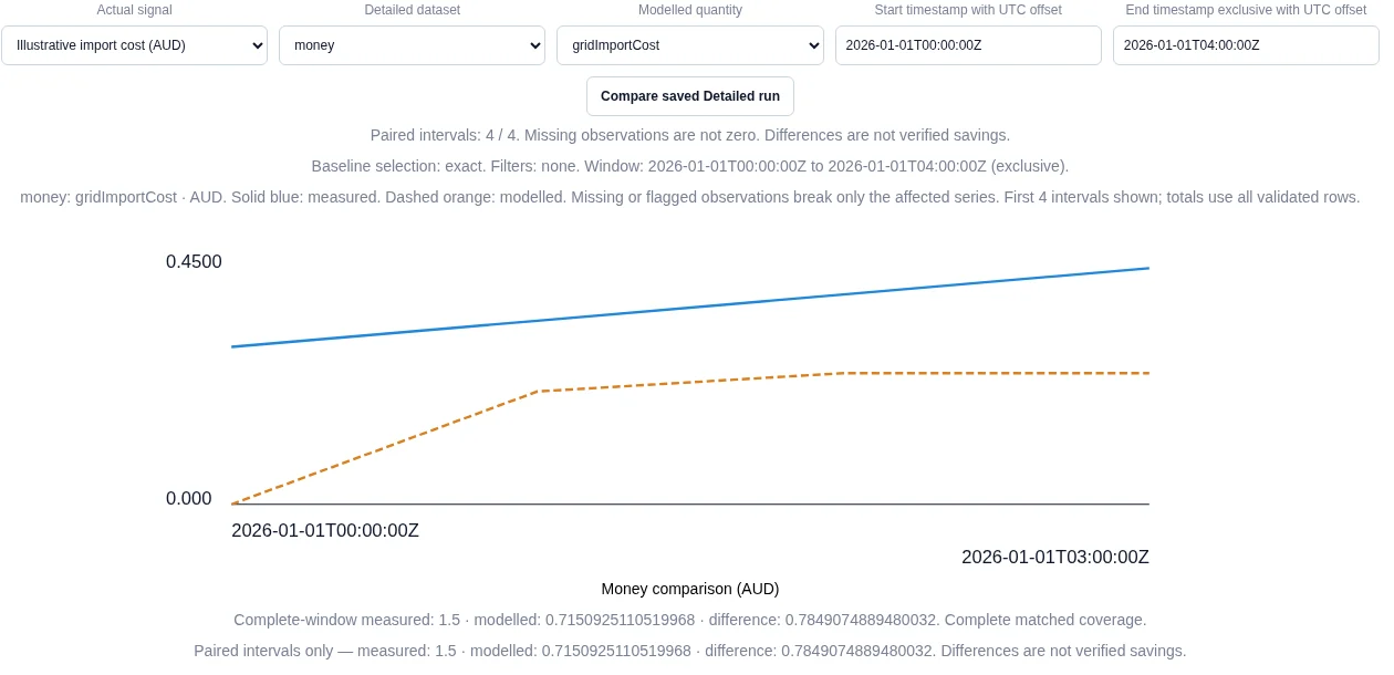
In Profiles → Saved Detailed run performance, select the completed run and your Actual signal. Choose money as the Detailed dataset and the matching Modelled quantity. Enter the comparison window, then select Compare saved Detailed run.
Worked example: four intervals, four allocation rows
We uploaded demonstration import costs of 0.30, 0.35, 0.40 and 0.45 AUD at hourly timestamps from 00:00 to 03:00 UTC on 1 January 2026. These are authored example inputs. Run f9386541be734188872aeeef2d4f513b saved host/owner shares of 60%/40% and solar/battery shares of 50%/50% for measured:gridImportCost.
The comparison window ended at 04:00 UTC, exclusive. The product showed Paired intervals: 4 / 4, measured money of 1.5 AUD (from the demonstration inputs), modelled money of 0.7150925110519968 AUD and a difference of 0.7849074889480032 AUD.
| 2026 allocation | Measured (AUD, demonstration inputs) | Modelled interval money (AUD) |
|---|---|---|
| host · solar | 0.45 | 0.214527753315599025 |
| host · battery | 0.45 | 0.214527753315599025 |
| owner · solar | 0.30 | 0.14301850221039935 |
| owner · battery | 0.30 | 0.14301850221039935 |