

Docs Menu
Dispatch Calendars and Sizing
Set operating bounds, test decision-price and forecast assumptions, and compare a small set of asset sizes in Project Modelling → Options.
Set a calendar bound
- Under Dispatch calendars, select Add calendar.
- Enter Name, Unit and Default value (blank = scalar bound).
- Select Add time window. Enter Months (1–12), Weekdays (Mon 0–Sun 6), Start minute, End minute and Value.
- Under Site limits, select the calendar for Site import calendar or Site export calendar.
- Save a case revision. Use aligned, timestamped profiles for a chronological run.
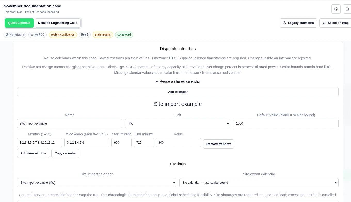
The example window is 10:00–12:00 in the displayed case timezone, UTC. All 12 months and all 7 weekdays are selected. These are example operating-limit assumptions. The scalar connection limit remains a hard limit.
Attach battery operating bounds
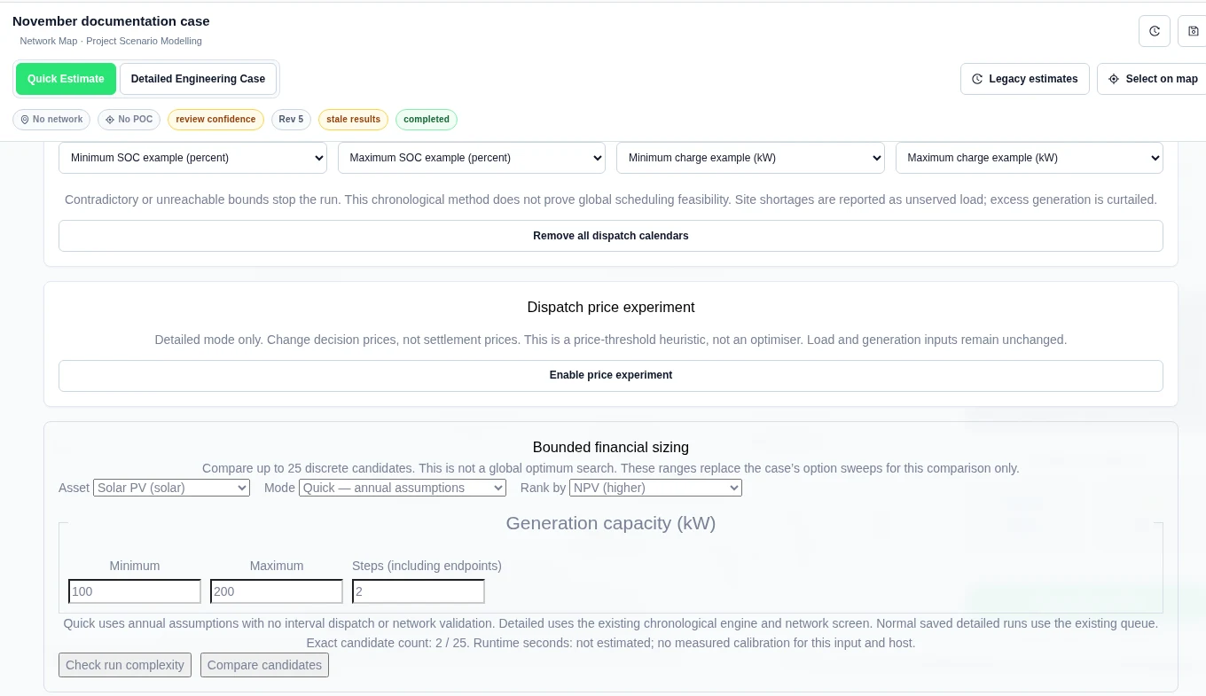
Add a Battery storage asset under Design first. Then return to Options. Use these four operating-bound selectors:
| Selector | Meaning |
|---|---|
| Minimum SOC / Maximum SOC | Percent of energy capacity at the end of an interval. |
| Minimum net charge / Maximum net charge | kW, or percent of rated power. Positive means charge; negative means discharge. |
Our configuration example selects 20% minimum SOC, 90% maximum SOC, −100 kW minimum net charge and 100 kW maximum net charge. These are input bounds, not a calculated dispatch result. The battery’s scalar limits still apply.
Reuse an exact library calendar
- In Profiles → Shared input library, create or select a dispatch_calendar item.
- Copy its pin: itemId, versionId and contentDigest.
- In Options, expand Reuse a shared calendar. Paste the pin into Calendar library pin JSON.
- Select Copy pinned calendar, then choose it in a site or battery selector.
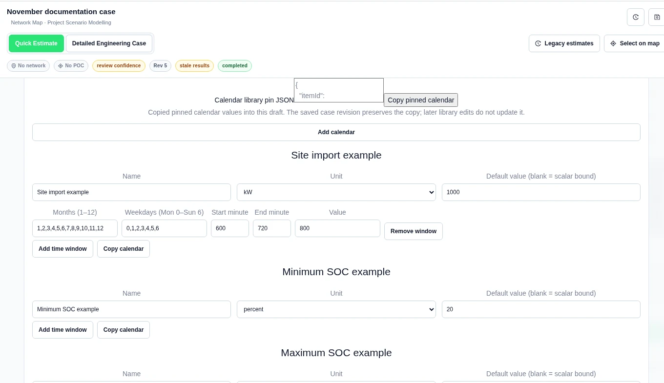
Our reusable Export ceiling calendar has unit kW, default 500 and no time windows. Copying it does not change the library. Later library edits do not update the case. Save a case revision to retain the copied values. A calendar ID must be unique in the case.
Set a decision-price experiment
- Under Dispatch price experiment, select Enable price experiment.
- Choose Price information and Threshold horizon.
- For Rolling elapsed hours, enter Rolling hours. Set Trailing smoothing intervals.
- Use a Detailed Engineering Case with suitable price inputs. Review results before retaining the assumption.
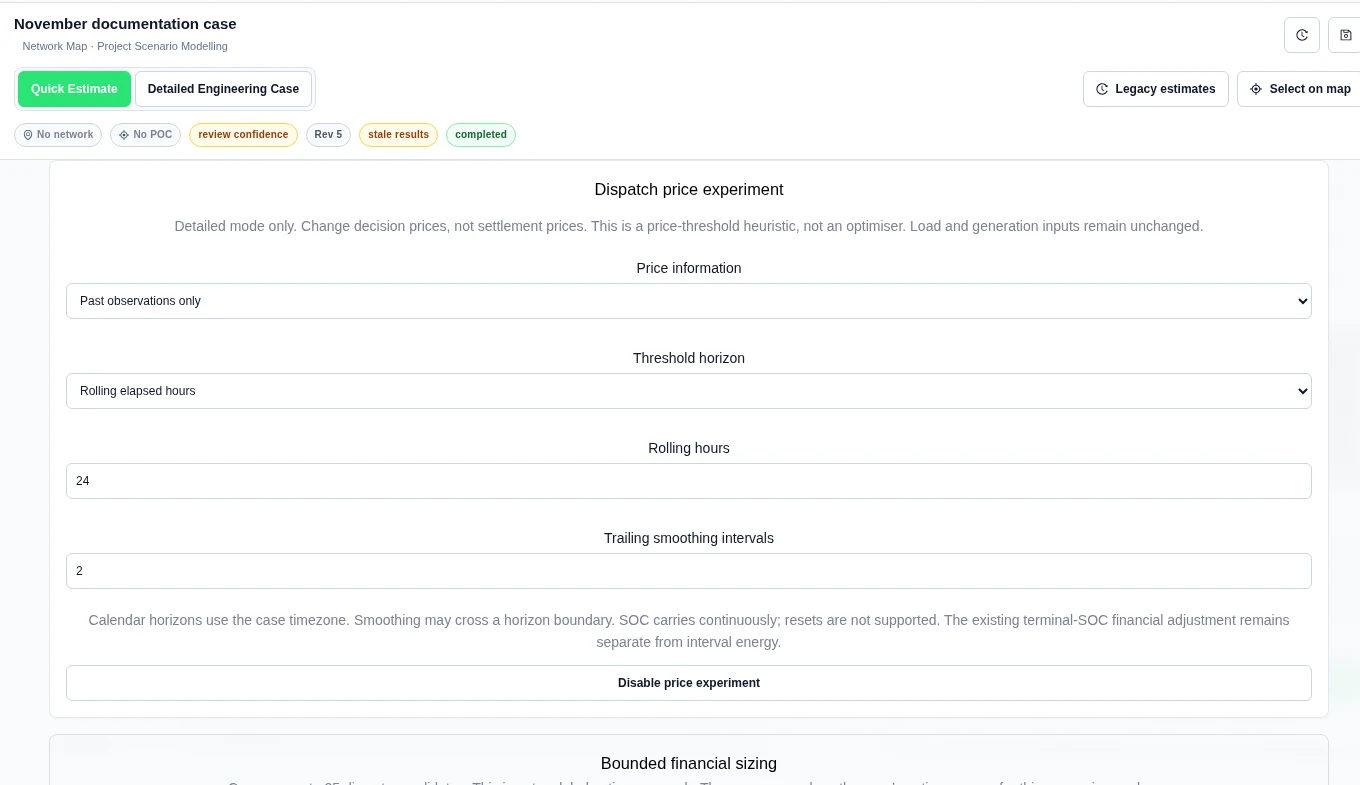
Perfect information — actual prices known in advance is an idealised assumption. Past observations only uses causal information. Calendar horizons use the case timezone. Smoothing can cross a horizon boundary. SOC carries continuously; it does not reset at each horizon.
This changes decision prices, not settlement prices, load or generation inputs. It is a price-threshold heuristic, not an optimiser. A supplied forecast needs a distinct, aligned price profile with explicit currency units and a valid frozen issue time; ordinary values alone are not enough. Use Disable price experiment to remove it.
Plan ahead with rolling look-ahead
- In Options → Dispatch price experiment, select Enable price experiment.
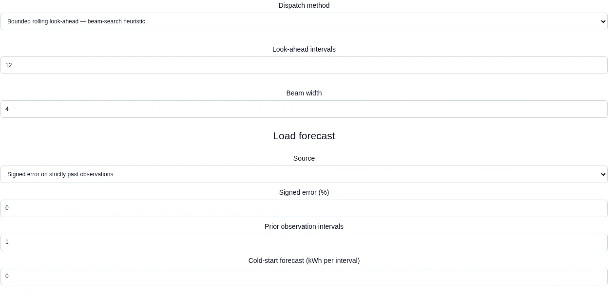
- Set Dispatch method to Bounded rolling look-ahead — beam-search heuristic. Enter Look-ahead intervals and Beam width.
- Choose the Source for Load forecast and Generation forecast. For Signed error on strictly past observations, set Signed error (%), Prior observation intervals and Cold-start forecast (kWh per interval).
- For supplied forecasts, select an aligned power or energy profile and its issue time. Save a case revision and run Detailed.
A signed forecast uses the mean of strictly earlier observations, multiplied by (1 + signed error / 100). The first decision uses the stated cold-start assumption. Current and future actuals are excluded. This is a user assumption, not a measured accuracy claim. Annual-normalised load and generation need supplied forecasts. Generation forecasts describe aggregate generation, not a capacity factor.
Price information is separate. Perfect information — actual prices known in advance still assumes future prices are known. Choose Past observations only for causal decision prices.
Keep SOC physical
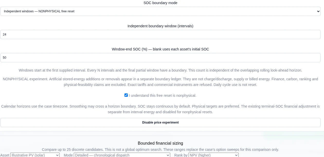
Continuous SOC — no reset (default) carries inventory forward. For a real end target, choose Physical window-end target — real energy required, then enter Independent boundary window (intervals) and Window-end SOC (%). Blank target SOC uses each battery's initial SOC. Real charge and discharge must meet all power, efficiency, SOC, connection and calendar limits.
Compare bounded sizes
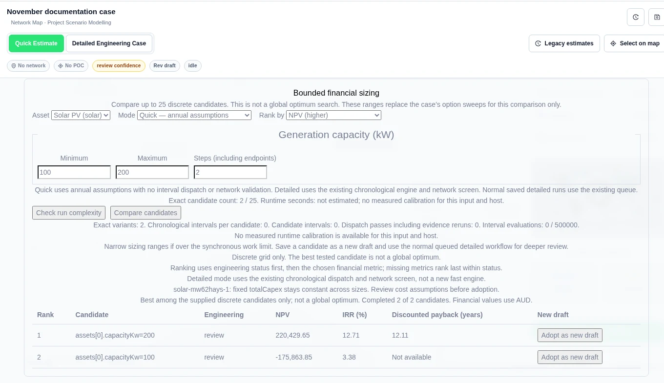
- Under Bounded financial sizing, choose Asset, Mode and Rank by.
- Enter Minimum, Maximum and Steps (including endpoints) for each size dimension.
- Select Check run complexity. Review the candidate count and work limit.
- Select Compare candidates. Read engineering status before the financial rank.
- For a candidate to retain, select Adopt as new draft. This creates a new saved draft; it does not replace the source case.
Worked example: two solar sizes
We selected solar, Quick — annual assumptions and NPV (higher). The range was 100–200 kW with 2 steps. The product completed 2 of 2 candidates:
| Capacity | NPV (AUD) | IRR | Discounted payback |
|---|---|---|---|
| 200 kW | 220,429.65 | 12.71% | 12.11 years |
| 100 kW | −175,863.85 | 3.38% | Not available |
The case used AUD, a 20-year horizon, 8% discount rate, 2.5% inflation, 2% energy and export escalation, and 2.5% opex escalation. Annual load was 1,000,000 kWh, peak demand 250 kW, solar yield 1,500 kWh/kW and degradation 0.5% a year. Import value was 0.25 AUD/kWh, export value 0.08 AUD/kWh and quick self-consumption 70%. Installed capex stayed at 500,000 AUD and annual opex at 5,000 AUD for both candidates. There was no replacement cost, network, point of connection or snapshot. Other value streams were zero. These were the model assumptions for the two-candidate comparison.
The product warned that fixed total capex stays constant across sizes. Review costs before adoption. We adopted the 200 kW candidate as a new draft.
Measure a sizing runtime estimate
- Set the sizing range and select Check run complexity.
- Select Measure runtime estimate (one candidate). This runs one real candidate; it is not a fixed speed claim.
- Read the measured projection and work counts before choosing Compare candidates.
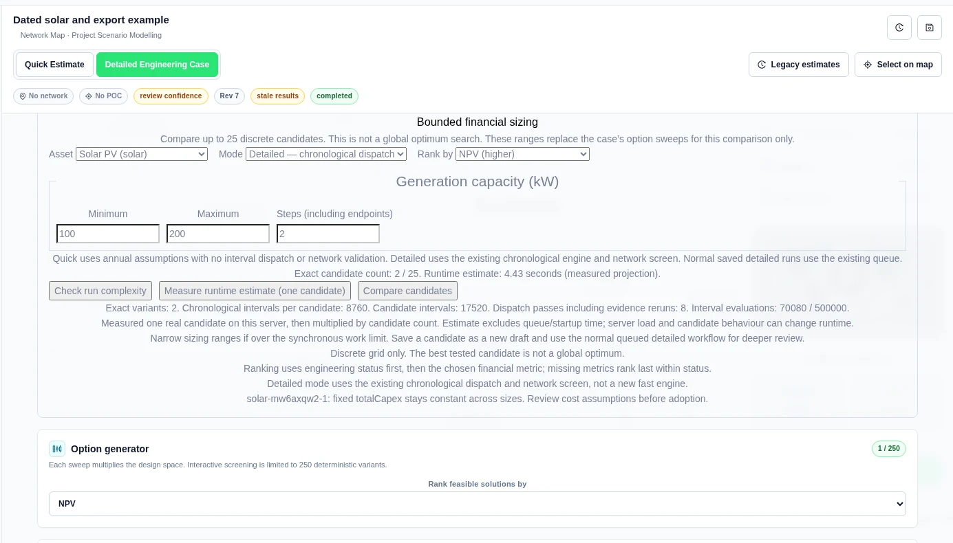
Our two-candidate Detailed example showed 4.43 seconds as its measured projection. The complexity result showed 8,760 intervals per candidate, 17,520 candidate intervals, 8 dispatch passes including evidence reruns, and 70,080 interval evaluations against a 500,000 limit. These are the actual counts for this example, not limits for all study types.
Use a fast sizing estimate
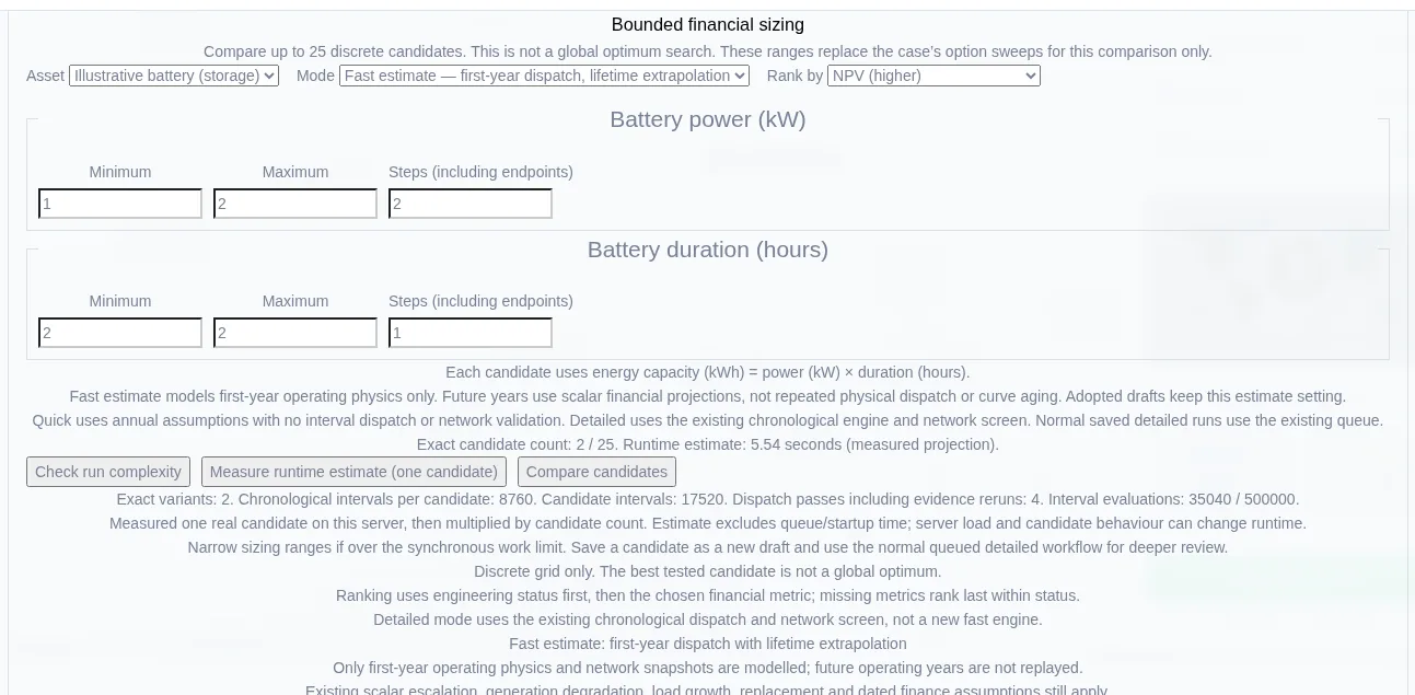
- Under Bounded financial sizing, set Mode to Fast estimate — first-year dispatch, lifetime extrapolation.
- Enter the size ranges.
- Select Measure runtime estimate (one candidate).
- Select Compare candidates.
- To use a size, choose a scenario in Apply sizes to scenario, or select Adopt as new draft. Save the case to keep applied sizes.
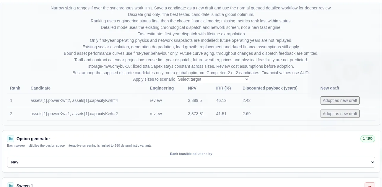
Worked example: two battery sizes
At North depot we chose the battery, power 1–2 kW in 2 steps, and duration 2 hours. The runtime estimate was 5.54 seconds (measured projection). Each candidate had 8,760 intervals, with 4 dispatch passes and 35,040 interval evaluations in total.
| Rank | Battery | NPV (AUD) | IRR | Discounted payback |
|---|---|---|---|---|
| 1 | 2 kW, 4 kWh | 3,899.5 | 46.13% | 2.42 years |
| 2 | 1 kW, 2 kWh | 3,373.81 | 41.51% | 2.69 years |
The product warned that the battery's fixed total capex stays the same across sizes. Check costs before you adopt a size.
Save a separate participant dispatch goal
- Open Value → Bounded participant dispatch.
- Enter Dispatch request JSON with explicit participants, selected parties, tariff rates and allocation fractions, interval timestamps and hours, fixed load, flexible-load bounds, required energy and import limits. Include currency and kW/kWh units.
- Set direction to minimize or maximize. Select Solve bounded dispatch.
- Read the objective, residual and Full dispatch result JSON.
- Select Apply bounded dispatch to case, then Save case revision, to retain this separate experiment.
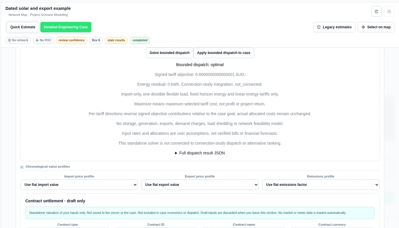
Worked example: minimise an allocated tariff cost
We supplied two one-hour UTC intervals on 1 January 2026. Each had 1 kW fixed load, flexible bounds 0–2 kW and a 3 kW import limit. Required flexible energy was 2 kWh. Energy rates were 0.1 and 0.5 AUD/kWh. The selected customer had 75% of the tariff; the owner had 25%.
The product returned optimal, with signed objective 0.60 AUD and energy residual 0 kWh. Applying and saving retained the request when we returned to the panel.
Use a participant goal in physical dispatch
- In Value → Participant value allocation, define and apply your participants.
- Leave Storage charging value blank to use the import rate. This is required for a case-energy goal and for joint optimisation.
- In Design, set storage Control policy to Tariff arbitrage.
- In Value → Physical dispatch goals, choose Case goal, the selected participants, each tariff's direction and explicit cost shares.
- Select Apply physical dispatch goals, then Save case revision. Run the Detailed Engineering Case.
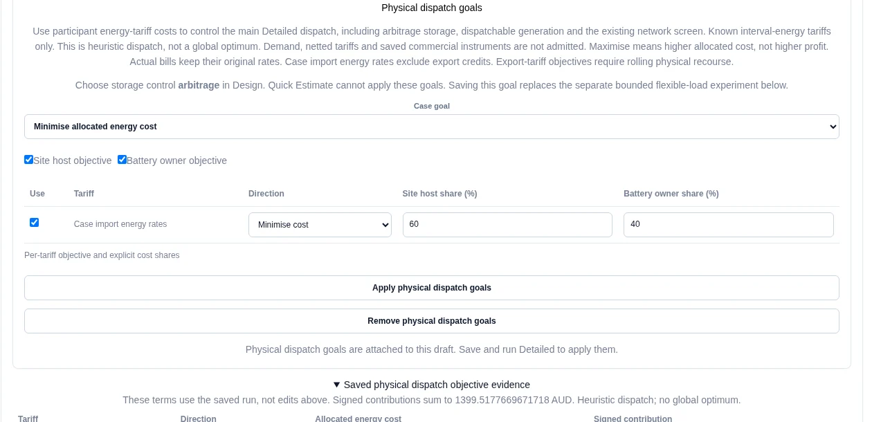
Unlike ordinary value allocation and the separate bounded flexible-load experiment, this goal changes main-case dispatch. Maximise allocated energy cost means higher cost, not higher profit. Actual bills retain their original rates. The default physical goal is heuristic dispatch, not a global optimum. Only supported interval-energy tariff goals are admitted; demand, netted tariffs and saved commercial terms need the separate joint path where supported.
Worked example: a saved case-energy goal
Our North depot case has 2 kW solar, a 2 kW / 4 kWh battery, 8,760 kWh annual load, import value 0.25 AUD/kWh and export value 0.08 AUD/kWh. Storage charging value was blank. We minimised both selected participants' case import energy cost with 60% and 40% shares.
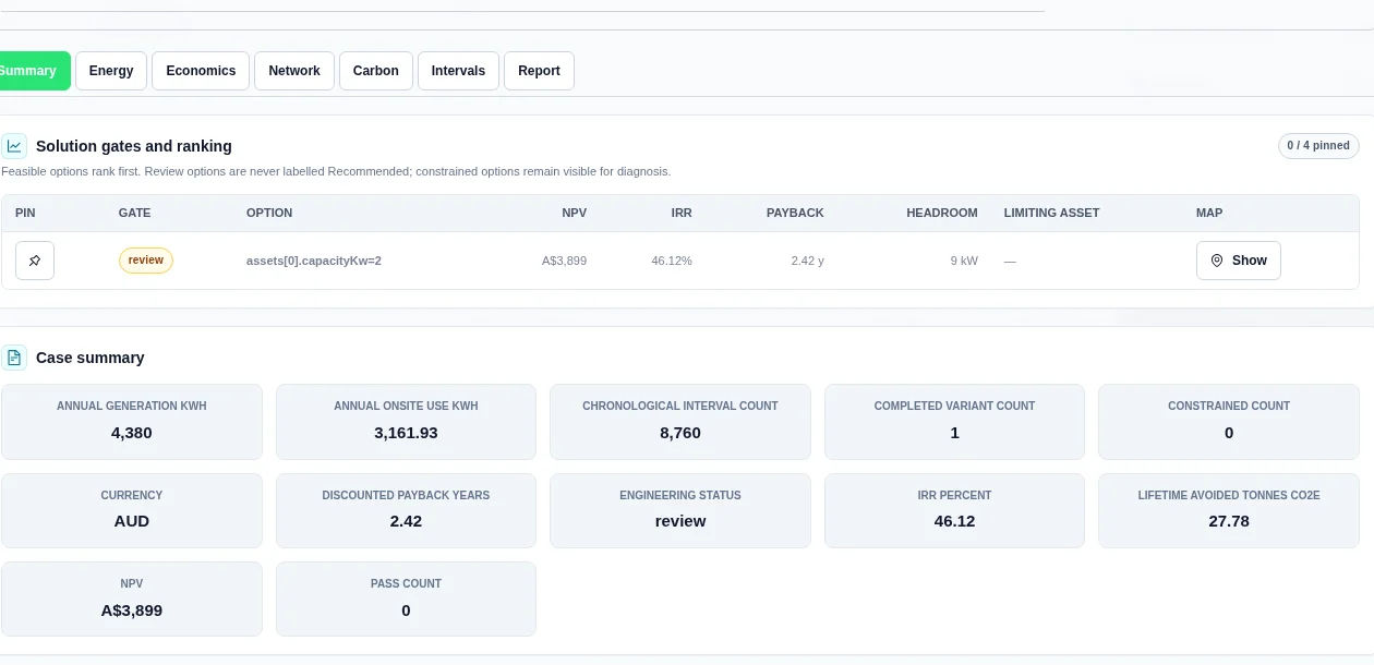
Saved physical dispatch objective evidence showed about 1,399.52 AUD as the signed contribution and allocated energy cost. The completed run showed 4,380 kWh generation, 3,161.93 kWh onsite use, 5,598.07 kWh import and 1,113.76 kWh export. NPV was A$3,899, IRR 46.12% and discounted payback 2.42 years. The engineering status remained review; no electrical network or POC was supplied.
Use joint Detailed optimisation
- Leave Storage charging value blank. Use exact tariff versions and save any commercial agreement version before pinning it.
- In Options, select Use joint optimisation in Detailed Analysis. Do not combine it with a forecast experiment.
- Save and run. In Results → Report, download the JSON manifest and inspect the joint-dispatch objective and diagnostics.

The joint model schedules multiple storage assets against shared import/export limits, efficiencies, SOC and calendar bounds, daily cycle budgets and a physical terminal SOC target. It uses known full-horizon inputs, not a forecast. Supported tariff rules, saved participant tariff shares and pinned commercial agreements can form one objective. Bounded demand formulas and decreasing demand blocks can shape the storage schedule. A selected participant objective can differ from whole-site economics.
Worked example: the same case with a physical terminal target
We cloned the participant-goal scenario and enabled joint dispatch. The saved objective artifact returned optimal, method joint_convex_lp (a linear optimisation with no yes/no decisions), objective about 1,399.85 AUD and the same tariff cost. There were no pinned contracts, so commercial settlement was 0. The results showed 4,380 kWh generation, 3,160.62 kWh onsite use, NPV A$3,301 and IRR 40.86%. This is not a like-for-like claim that one dispatch method always earns more: the joint model enforces a physical terminal inventory.
Worked example: rolling demand and decreasing blocks
We supplied four one-hour intervals on 1 January 2026 in UTC. The example load was 0, 3, 0 and 1 kW. A 1 kW / 2 kWh battery started and ended at 50% SOC. Both efficiencies were 100%. The import limit was 3 kW and the export limit was 0 kW.
With a two-interval rolling demand formula and an example rate of 20 AUD/kW, the saved objective was 20 AUD. Exact settlement was also 20 AUD. The saved method was joint_convex_lp and status was optimal.
We then used decreasing demand blocks: the first 0.5 kW at 8 AUD/kW, the next block up to 1.5 kW at 2 AUD/kW, and the remaining demand at 1 AUD/kW. The saved method was joint_bounded_milp, with 2 integer variables. This method is used when the problem needs yes/no (integer) decisions, such as demand blocks. The objective and exact settlement were both 6.5 AUD. Each example covers only its four supplied intervals.
In the JSON manifest, inspect joint-dispatch-objective. It records the method, status, tariff terms and exact-settlement reconciliation. The rolling and decreasing-block examples both returned a reconciliation difference of 0 AUD.
Run a NONPHYSICAL SOC reset experiment
- In Options, select Enable price experiment. Choose Bounded rolling look-ahead — beam-search heuristic.
- Supply valid load, generation and price forecasts. Set SOC boundary mode to Independent windows — NONPHYSICAL free reset.
- Set the independent window length and window-end SOC. Acknowledge the warning. Save and run.
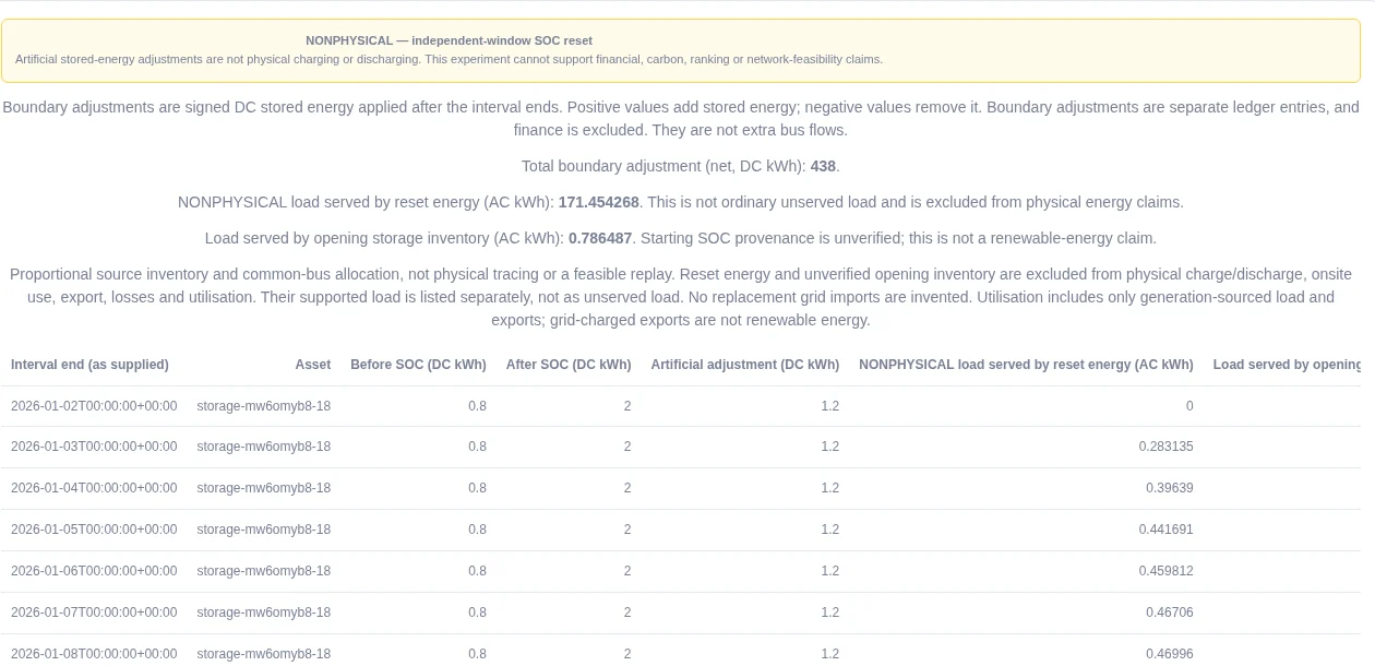
- In Results, read the NONPHYSICAL banner, total adjustment and SOC boundary adjustments ledger. Check Energy and Economics separately.
Worked example: separate artificial support from physical energy
We reran the North depot reset scenario over 8,760 hourly intervals in 2026. The battery was 2 kW / 4 kWh. Look-ahead was 12 intervals, beam width 4, and load forecast used one prior observation, 0% signed error and a 0 kWh cold start. Generation used a separate assumed frozen 1 kW forecast issued on 31 December 2025. Actual solar generation remained the supplied resource profile. Annual load normalisation was off.
The product reported a net adjustment of 438 DC kWh. Each boundary added 1.2 DC kWh, taking simulated SOC from 0.8 to 2 kWh. Reset-supported load was about 171.45 AC kWh. Opening-inventory support was about 0.79 AC kWh. These are separate references, not ordinary unserved load or renewable supply.
| Full-horizon result | Product value |
|---|---|
| Generation | 4,380 kWh |
| Physical onsite use | about 2,068.33 kWh |
| Physical export | about 2,311.67 kWh |
| Renewable utilisation | 100% |
Onsite use plus export equals generation in this example. The energy preview reconciled all 2,000 returned intervals. That preview is capped; the summary covers all 8,760 simulated intervals. A full simulated horizon is not always a full calendar year.
Economics showed: “Finance excluded: Nonphysical independent-window SOC reset; artificial energy cannot support financial or carbon claims.” NPV and IRR were unavailable, not zero.

Plan fleet charging
Open Design and find Mobility planning. Enter the fleet in Fleet plan JSON. Give each vehicle its usable energy, opening energy, reserve and departure requirement. Add charger groups, dated connection sessions and site import and export limits.
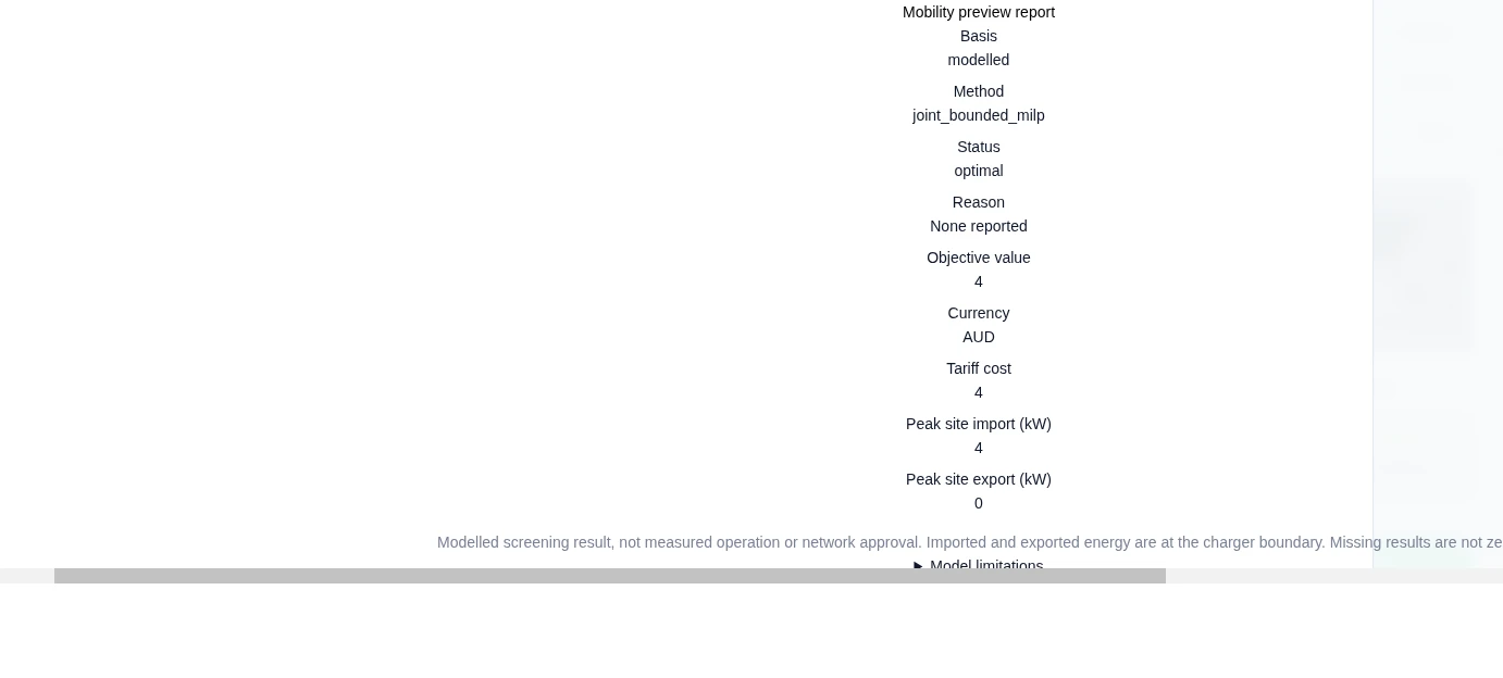
In Preview profiles JSON, enter the interval timestamps, load, generation and import and export prices. Select Preview mobility dispatch. The Mobility preview report shows the modelled schedule, tariff cost and vehicle energy balance.
In this two-hour example, one vehicle starts empty and needs 4 kWh at departure. Its charger limit is 4 kW. Import prices are 1 then 2 AUD/kWh. The preview charges 4 kWh in the first hour and none in the second. The tariff cost is 4 AUD, closing energy is 4 kWh, and departure shortfall is 0 kWh.
Model bidirectional charging
Choose the bidirectional mode in the fleet plan. Supply vehicle consent and an export permission record with its dates, power limit and evidence reference. The schedule uses these caller-supplied assumptions together with the vehicle reserve and discharge efficiency.
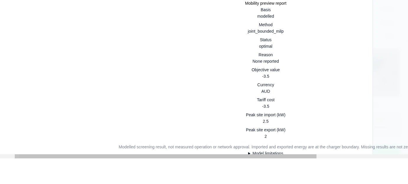
In the second example, the vehicle starts and finishes at a 4 kWh reserve. Discharge efficiency is 80%, the export limit is 2 kW, and the second-hour export price is 3 AUD/kWh. The preview imports 2.5 kWh, exports 2 kWh and records 0.5 kWh of loss. Its modelled tariff cost is −3.5 AUD, with no departure shortfall.
Inspect Vehicle energy totals and Interval dispatch for the charge, discharge and state of charge. Use Apply mobility plan to draft to carry the plan into the case. Save the case and use Detailed Analysis with joint optimisation for the case run.
Apply connection access limits
Open Design and find Scheme sources and connection access. Under Explicit connection agreement, enter Connection preview JSON. Supply the agreement reference and digest, timezone, dates, import and export permission, rating and agreement caps. Add dated instructions or an access calendar for the study.
Select Preview access limits. The table shows import and export limits for each UTC interval, with the constraint that sets each limit. Use Apply access attachment to draft to keep the agreement inputs with the case.
This three-hour example has a 100 kW import rating, split into 40 kW firm and 60 kW flexible access, and a 90 kW agreement cap. Supplied instructions of 200, 20 and 60 kW produce modelled import limits of 90, 20 and 60 kW. The example has no export permission, so its export limit is 0 kW in all three intervals.



