

Docs Menu
Connection Study and System Feasibility
Use System Feasibility to screen solution types, then use Connection Study to compare fixed designs at one point of connection.
Watch the Video: Connection Studies & Hosting Capacity (1:40)
Choose the right study
Open Engineering Studies, then choose System Feasibility or Connection Study. These workbenches require Professional or Enterprise access.
| Tool | Use it for | Important boundary |
|---|---|---|
| System Feasibility | Record project needs, inspect map and profile evidence, and compare solution types. | Use the preliminary recommendation to scope the next modelling step. |
| Connection Study | Compare a reference case with fixed solar, battery, flexible-load, and targeted-network-work alternatives at a shared point of connection. | It optimises dispatch. It does not search for the best equipment size. |
| Project Scenario Modelling | Develop the project model, resource sizes, dispatch, and financial assumptions. | Use its engineering follow-on studies to test the selected design. |
| Power Planning | Run chronological dispatch, unit commitment, capacity expansion, resource adequacy, two-stage stochastic or hydro studies on a planning case. See Power Planning. | Results show planning-model outcomes for the inputs you supply. The PLEXOS 12 package is export only and is a compatibility candidate. A PLEXOS licence is not included. |
| Hosting Capacity | Screen additional distributed energy resource capacity in a selected network model. | Review the tested capacity range and the limiting conditions in the selected model. |
For the full System Feasibility procedure, see System Feasibility and Planning Studies.
Start a Connection Study
- Open Connection Study.
- Complete Scope and Profiles.
- Define fixed designs in Alternatives.
- Add shared conditions in Stress Cases.
- Review Value and Optimise.
- Use Run to check readiness and submit the selected alternatives.
- Inspect Results before making a recommendation.
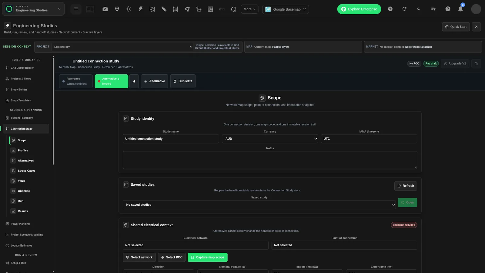
Scope and shared electrical limits
All alternatives use the same electrical network, point of connection, reference profiles, limits, tariff, and finance basis.
| Field or action | Meaning and initial value |
|---|---|
| Study name and Notes | Identify the study and record assumptions. |
| Currency | AUD initially. Also supports USD, NZD, EUR, and GBP. This labels monetary inputs; it does not convert entered amounts. |
| IANA timezone | UTC initially. Use the timezone that applies to the chronological data and tariff. |
| Electrical network and Point of connection | Selected map context. Use Select network and Select POC to change it. |
| Capture map scope | Capture an immutable snapshot of the current scope. Use Done selecting or Return to study to leave map selection. Capture a new snapshot after changing the network or point of connection. |
| Direction | Import and export initially. Alternatives are Import only and Export only. |
| Nominal voltage | 11 kV in a default draft without supplied context. |
| Import limit and Export limit | 5,000 kW each in a default draft without supplied context. |
| Minimum voltage and Maximum voltage | 0.95 pu and 1.05 pu initially. Maximum must exceed minimum. |
| Maximum thermal loading | 100% initially. Enter a positive limit. |
| Allow reverse power flow | Enabled initially. Review this permission for the selected connection. |
Attach chronological profiles
- Open Profiles.
- Set Profile scaling peak demand. The initial value is 250 kW.
- Set Reference load power factor. The initial value is 0.95. It must be greater than zero and no greater than one.
- Select a Profile type.
- Check Unit.
- Choose a CSV/XLSX file.
- Select Validate and attach.
- Check the attached profile's interval, unit, and validation status.
- Select the required Load profile. Select an optional Existing generation profile, or leave it as None.
| Profile type | Initial unit | Use |
|---|---|---|
| Load | kW | Reference demand chronology. |
| Generation | kW | Existing generation chronology. A normalized generation profile can also serve solar availability when its unit and values are suitable. |
| Availability | fraction | Solar availability. Use a normalized 0–1 series. |
| Tariff / market | Selected currency/kWh | Time-varying import or export energy prices. |
| Emissions | kgCO2e/kWh | Time-varying grid emissions intensity. |
Use a header row with timestamp and value columns for a clear upload layout. XLSX uploads read the first worksheet. CSV data uses UTF-8 encoding and accepts comma, semicolon, tab, or pipe delimiters. The file limit is 25 MB. The table parser also limits inputs to 1,000,000 data rows and 2,000 columns; an XLSX workbook must not exceed 250 MB after decompression. Supported intervals are 5, 10, 15, 30, and 60 minutes; the uploader infers the interval from timestamps. Validation checks full-year coverage, gaps, duplicate timestamps, and increasing timestamp order.
Files must contain usable chronological timestamps and numeric values. Referenced profiles must have valid status. warning means issues such as incomplete annual coverage need attention. invalid indicates failures such as duplicate, unparseable, or non-increasing timestamps. Neither warning nor invalid profiles satisfy the run requirement. Resolve timestamp, unit, missing-value, or interval issues before running. Do not replace missing measurements with zero merely to pass a check. Use the remove control on a profile card to detach an unwanted profile, then check any selectors that referenced it.
A solar alternative needs a valid availability profile, or a normalized generation profile in fraction, pu, or p.u. units. An ordinary generation series in kW is not a normalized availability series.
Set tariffs and financial assumptions
Value uses the applicant perspective. The same assumptions apply to the reference and every alternative.
| Field | Initial value and unit | Purpose |
|---|---|---|
| Demand billing period | Monthly; optional Annual | Select the period for the demand charge. |
| Demand rate | 0 currency/kW-month, or currency/kW-year for annual billing | Price of billed peak demand. |
| Fixed annual charge | 0 currency/year | Annual fixed tariff cost. |
| Grid services revenue | 0 currency/year | Assumed annual service revenue. |
| Storage capacity revenue | 0 currency/kW-year | Assumed battery capacity revenue rate. |
| Analysis horizon | 20 years | Financial assessment period. |
| Discount rate | 8% | Discount future cash flows. |
| Inflation | 2.5% | Shared inflation assumption. |
| Energy escalation | 2%/year | Energy-price escalation assumption. |
| OPEX escalation | 2.5%/year | Operating-cost escalation assumption. |
| Import emissions factor | 0.65 kg CO2-e/kWh | Flat grid emissions intensity when no emissions profile is selected. |
| Carbon value | 0 currency/t CO2-e | Value assigned to emissions reduction. |
| Emissions profile | Use flat factor | Select a valid attached emissions profile to use a time-varying factor instead. |
Import and export energy tariffs
Choose one Rate source separately for import and export.
| Source | Inputs |
|---|---|
| Flat rate | Set Import energy rate and Export energy rate as applicable. Initial rates are 0.25 and 0.08 currency/kWh. |
| Market profile | Select a valid attached Market profile in the correct price unit. |
| Time of use | Use Add import period or Add export period. Enter each period and remove unwanted periods with its remove control. |
Each time-of-use period has Name, Months, Weekdays, Start minute, End minute, and Period rate. Enter months as comma-separated numbers from 1 to 12. Enter weekdays as numbers from 0 (Monday) to 6 (Sunday). The time window uses minutes after midnight: 0 is the start of the day and 1440 is its end. A new period initially covers all months, all weekdays, and the full day. Set the actual windows and rates before running.
Read the value ledger
Value ledger shows Value stream, Treatment, and Rate for the active alternative. Benefits include avoided grid imports, export revenue, demand-charge reduction, grid services, storage capacity revenue, and carbon value. Costs include fixed charges, installed capital cost, and operating cost. Derived means the amount comes from the design or result rather than a standalone rate. The run-level value_ledger dataset contains annual rows.
Save, reopen, or upgrade
- Use the save control labelled Save Connection Study revision to store an immutable revision. The header shows an unsaved draft or the saved revision.
- In Saved studies, select Refresh, choose a Saved study, and select Open. This opens its latest revision. It also restores a run for that revision when one is available, and loads its results if the run completed.
- Upgrade V1 is available when a saved first-generation feasibility case is open. It creates a Connection Study from that case and its selected solution. Review the transferred inputs before running.
Check readiness and run
- Open Optimise. The Objective is Applicant NPV. The Solver is HiGHS.
- Review Dispatch time limit. It starts at 900 seconds; the form minimum is 30 seconds.
- Open Run.
- Resolve every blocking readiness message. Checks include shared context, snapshot, profiles, positive equipment sizes, valid storage SOC bounds, valid work targets, tariff inputs, finance inputs, and stress multipliers.
- Choose Validation mode: Screen — broad comparison or Finalists — recommendation eligible.
- Pin the alternatives to compare with Add to comparison.
- Select Save & preflight. Review the backend status and estimated work. Resolve blocking inputs before continuing.
- Select the run button. Its label shows the number of selected alternatives.
- Wait for completion. Inspect the run status and progress. If the run fails, review its message, correct the inputs, and submit again.
Use a valid timezone, electrical network, point of connection, and captured snapshot. Supply at least one configured design. Set import and export limits and flat tariff rates to nonnegative values. Select a valid market profile for a profile-based rate, or add periods for a time-of-use rate. Use a positive analysis horizon and a nonnegative discount rate. Fix any field-specific messages before continuing.
Readiness checks the study's configured alternatives, not only the pinned subset. After preflight, run the study to review the engineering checks. Queued means the request is waiting; running means processing is in progress; completed means results are available; failed means the run did not complete successfully.
See Connection Study Alternatives and Recommendations for design inputs, stress tests, result interpretation, and recommendation gates.
Related Guides
- Project Modelling
- System Feasibility and Planning Studies
- Connection Study Alternatives and Recommendations
- Hosting Capacity Screening
- Project Modelling tariffs
- Project Modelling value and finance


