

Docs Menu
Value and Finance
Set project values and costs, then read the financial results from the same saved case and run.
Before you start
Open Value & Finance in Project Scenario Modelling. Engineering Studies requires Professional or Enterprise access. Complete the scope, profiles, and asset design first.
The workbench uses unlevered project cash flows. Debt, tax, and depreciation are outside this assessment. Replace the default assumptions with the prices and costs for your project.
- Check the case Currency. The choices are AUD, USD, NZD, EUR, and GBP. A new workbench case defaults to AUD unless its context supplies another currency.
- Enter asset capital and operating costs in DER Design.
- Set the study horizon and value assumptions.
- Apply a network tariff or enter rates manually.
- For Detailed assessment, select validated price and emissions profiles if needed.
- Save the case revision and run the assessment.
- Review the metric cards in Economics and Carbon.
Step 4 inputs and defaults
These are new workbench-case defaults. Monetary defaults below use the case currency. Escalation applies from the second year. The first year uses the entered rate.
| Field | New-case default | Purpose |
|---|---|---|
| Analysis horizon | 20 years | Number of years in the project cash-flow assessment. |
| WACC / discount rate | 8% | Rate used to discount future cash flows and lifecycle costs. |
| Inflation | 2.5% | General inflation assumption recorded with the case. Set the specific escalation rates below for the cash-flow model. |
| Energy escalation | 2% per year | Annual escalation of the import energy value. |
| Export escalation | 2% per year | Annual escalation of the export energy value. |
| Opex escalation | 2.5% per year | Annual escalation of operating costs. |
| Import energy value | 0.25 per kWh | Value of grid electricity avoided by the project. |
| Export energy value | 0.08 per kWh | Value of energy exported to the grid. |
| Storage charging value | 0.15 per kWh | Grid charging cost assumption. Quick assessment uses it for grid charging; Detailed assessment also uses it in storage cost calculations. |
| Demand value | 0 per kW/month | Value of reducing grid demand. The monthly rate is multiplied by 12 for the annual calculation. |
| FCAS / capacity revenue | 0 per year | Annual grid-service revenue assumption, separate from energy sales. |
| Generation capacity value | 0 per kW/year | Annual capacity value applied to generation capacity. |
| Fixed annual charge | 0 per year | Fixed tariff assumption recorded with the case. Check the cash-flow output when assessing total bill costs. |
| Quick self-consumption assumption | 70% | Share used by the Quick annual energy estimate. Detailed assessment uses chronological dispatch instead. |
| Emissions factor | 0.65 kg CO₂-e/kWh | Flat factor for avoided emissions. |
| Carbon value | 0 per t CO₂-e | Value assigned to avoided emissions. |
| Decommissioning cost | 0 | Project end-of-life cost, in the case currency. |
The analysis horizon must be greater than zero. The saved model supports 1–50 years. The workbench requires a discount rate of zero or greater. Keep the self-consumption percentage between 0 and 100. Correct validation messages before running.
Asset costs and lifecycle
Each asset has Installed capex, Annual opex, Annual degradation, Replacement year, Replacement cost, and Decommissioning cost. See DER Design for the asset fields and units.
- Installed capex is paid at the start of the assessment.
- Annual opex contributes to operating cost. Biomass fuel cost also contributes to operating cost.
- Replacement cost is a percentage of the asset capex, applied in the selected replacement year.
- Decommissioning is a final-year cost. Check both the asset and case-level entries so that the same cost is not entered twice.
- Degradation reduces modelled energy over the assessment horizon. It is separate from price escalation.
How value is calculated
Energy and demand
Quick assessment values annual onsite energy at the import value and exported energy at the export value. It deducts the modelled grid-charging cost. Detailed assessment compares baseline and project import costs and export revenue using chronological energy flows.
Quick demand reduction is a screening estimate based on generation capacity, the self-consumption assumption, storage power, and modelled peak demand, including load adjustments. Detailed demand reduction is the positive difference between baseline peak demand and modelled peak grid import. Annual demand savings equal demand reduction in kW × monthly demand value × 12.
Services, capacity, and carbon
FCAS / capacity revenue adds an annual service-value assumption. It does not simulate dispatch into a frequency control ancillary services market or confirm eligibility for payment. Generation capacity value multiplies the entered annual value by generation capacity.
Carbon value equals avoided emissions in tonnes CO₂-e × value per tonne. A zero carbon value leaves the emissions result available without adding carbon revenue.
Market prices and loss factors
Import price profile and Export price profile select uploaded Market / value profiles. The flat alternatives are Use flat import value and Use flat export value. Emissions profile selects an emissions profile; Use flat emissions factor retains the entered factor.
Chronological profiles support Detailed assessment. The market-profile upload defaults to case currency/MWh. Price series in currency/MWh are converted to currency/kWh for energy calculations. Check units, timestamps, and coverage before use. See Profiles and Inputs for CSV and XLSX upload instructions.
Keep the price basis consistent with your settlement assumptions. These inputs do not automatically attach a marginal loss factor to a generating unit. For the separate unit-revenue workflow, see Unit Revenue with Loss Factors.
Financial and carbon metrics
| Metric | Meaning |
|---|---|
| Total capex | Sum of the modelled asset capital costs. This is the initial project investment. |
| First-year revenue and savings | Energy value, demand savings, service revenue, generation capacity value, and carbon value before operating and replacement costs. |
| First-year opex | First-year asset operating costs, including modelled fuel costs. |
| NPV | Net present value in the case currency. A positive value means discounted modelled benefits exceed discounted modelled costs at the selected discount rate. |
| IRR | Discount rate at which the modelled cash flows have zero NPV, expressed as a percentage. A result is not available when the solver cannot find a valid rate. |
| Discounted payback | Years until cumulative discounted cash flow first recovers the initial investment. The calculation interpolates within the recovery year. No result means recovery was not found within the horizon. |
| LCOE | Levelized cost of energy: discounted project lifecycle costs divided by discounted generation, in currency/kWh. Detailed assessment uses new project generation in the denominator. |
| LCOS | Levelized cost of storage: discounted storage costs divided by discounted storage discharge, in currency/kWh. No positive discharge means this metric is not available. |
| First-year avoided emissions | Avoided emissions in kg CO₂-e for the first modelled year. |
| Lifetime avoided emissions | Sum of modelled avoided emissions over the horizon, in t CO₂-e. |
| First-year carbon value | First-year avoided kg CO₂-e divided by 1,000, then multiplied by the carbon value per tonne. |
Cash-flow formulas
Let C₀ be initial capex, CFᵧ be net cash flow in year y, r be the discount rate divided by 100, and N be the analysis horizon.
- Net cash flow = revenue and savings − operating cost − replacement cost − any final-year decommissioning cost.
- Discounted cash flow in year y = CFᵧ / (1 + r)ʸ.
- NPV = −C₀ + sum of discounted cash flows for years 1 through N.
- Cumulative discounted cash flow starts at −C₀ and adds each year's discounted cash flow.
- IRR is a rate for which the NPV formula equals zero.
LCOE includes capex and discounted operating, fuel, replacement, and decommissioning costs. It does not deduct energy revenue from that cost numerator. LCOE is not available without positive discounted generation.
LCOS cost scope depends on the assessment mode. Quick assessment includes storage capex, operating costs, and replacement costs. Detailed assessment also includes grid charging, terminal state-of-charge replenishment, and storage decommissioning. Compare LCOS only after checking the mode and cost scope.
Economics result cards
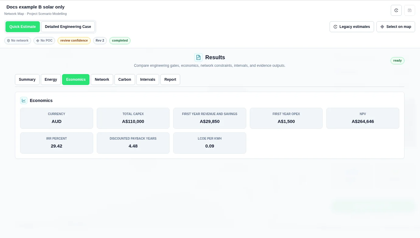
The Economics tab shows metric cards, including capex, first-year revenue and savings, first-year opex, NPV, and available return and payback metrics. Open Cashflow explorer below the cards to inspect and export the supplied cash flows. The formulas above explain how the model calculates its financial metrics.
Legacy Estimates has separate Cumulative Cash Flow and Annual Cash Flow charts. These charts belong to the legacy calculator, not the versioned case results. They are not an annual cash-flow table.
One value per design, not one value per year
To compare designs on the same load, prices, horizon and discount rate, use the ranked NPV chart in Results → Summary. Each column is a whole design’s NPV in the case currency. A value below zero means the modelled benefits fall short of the costs at that discount rate. Use Cashflow explorer instead to see when costs and benefits occur.
In the Riverbend cold store example, three solar sizes are paired with three battery sizes. The plot ranks the nine designs but does not certify a connection or forecast a return.
Economics example
Legacy estimate finance
Legacy estimates uses a separate annual estimate in the browser. It is not the same calculation as a versioned Engineering Case. Legacy money outputs use USD formatting; there is no currency conversion.
| Field | Default | Use |
|---|---|---|
| Initial Investment | 10,000 | Initial capital outflow. |
| System Lifespan (years) | 20 years | Length of the annual cash-flow calculation. |
| Electricity Rate | 0.10 per kWh | Avoided import value in flat-rate mode. |
| Feed-in Tariff | 0.05 per kWh | Value of exported generation. |
| Discount Rate / WACC (%) | 8% | Discount rate for NPV and discounted payback. |
| O&M (% of capex) | 1% per year | Annual operating cost as a share of the initial investment. |
| Inflation Rate (%) | 2% | Part of the combined annual value escalation. |
| Escalation Rate (%) | 2% | Added to the inflation rate for annual value escalation. |
| Decommissioning (% of capex) | 5% | Cost deducted in the final year. |
| Replacement Cost | 5,000 | Battery replacement cost when storage is included. |
| Replacement Interval (years) | 10 years | Repeat the replacement cost at each interval within the study horizon. |
| Battery Operation | Coordinated with generation | Use an import/export or peak/off-peak spread. Independent arbitrage uses the separate battery tariff value. |
| Battery Tariff | 0.05 per kWh | Value per unit of estimated battery throughput in independent mode, not a charging-cost input. |
| Include FCAS revenue | Off | Include the annual service revenue only when battery storage is included. |
| Annual FCAS Revenue | 1,000 per year | Flat annual revenue when the FCAS option is enabled. |
| Solar Capex ($/kW) | 1,200 per kW | Unit capital cost used by the legacy solution finder. |
| Battery Capex ($/kWh) | 800 per kWh | Unit storage capital cost used by the legacy solution finder. |
The legacy annual value multiplier is (1 + inflation rate + escalation rate) raised to year minus one. Rates in this formula are percentages divided by 100. It escalates energy value, battery value, demand savings, and fixed charges. Annual O&M remains the entered percentage of initial investment. FCAS revenue is a flat annual assumption.
The legacy cash flow adds onsite energy value, export value, battery value, demand savings, and enabled FCAS revenue. It subtracts O&M, fixed tariff charges, battery replacements, and final-year decommissioning. Legacy Payback is discounted payback. Not reached means the investment was not recovered within the selected horizon. N/A for IRR means no valid rate was found.
See the tariff guide for the legacy flat and weighted time-of-use rates. Use Upgrade to Engineering Case when you need versioned inputs, engineering assessment, and presentation export.
Contract valuation and participant shares
Contract settlement · draft only is the standalone calculator. It does not save its draft or add its result to case economics. The separate Saved commercial instruments panel saves immutable versions and pins them to a case for post-dispatch settlement. It does not change physical dispatch. See Contract Settlement for the workflow and limits.
Participant value allocation splits signed source cash flows by percentage. The unassigned share remains visible. Apply the allocation, save a revision and re-run before reading saved results. See Participant Allocation.
The Shared Library also quotes dated cost rate cards. A quote does not fill case costs automatically.
Inspect annual cash flows
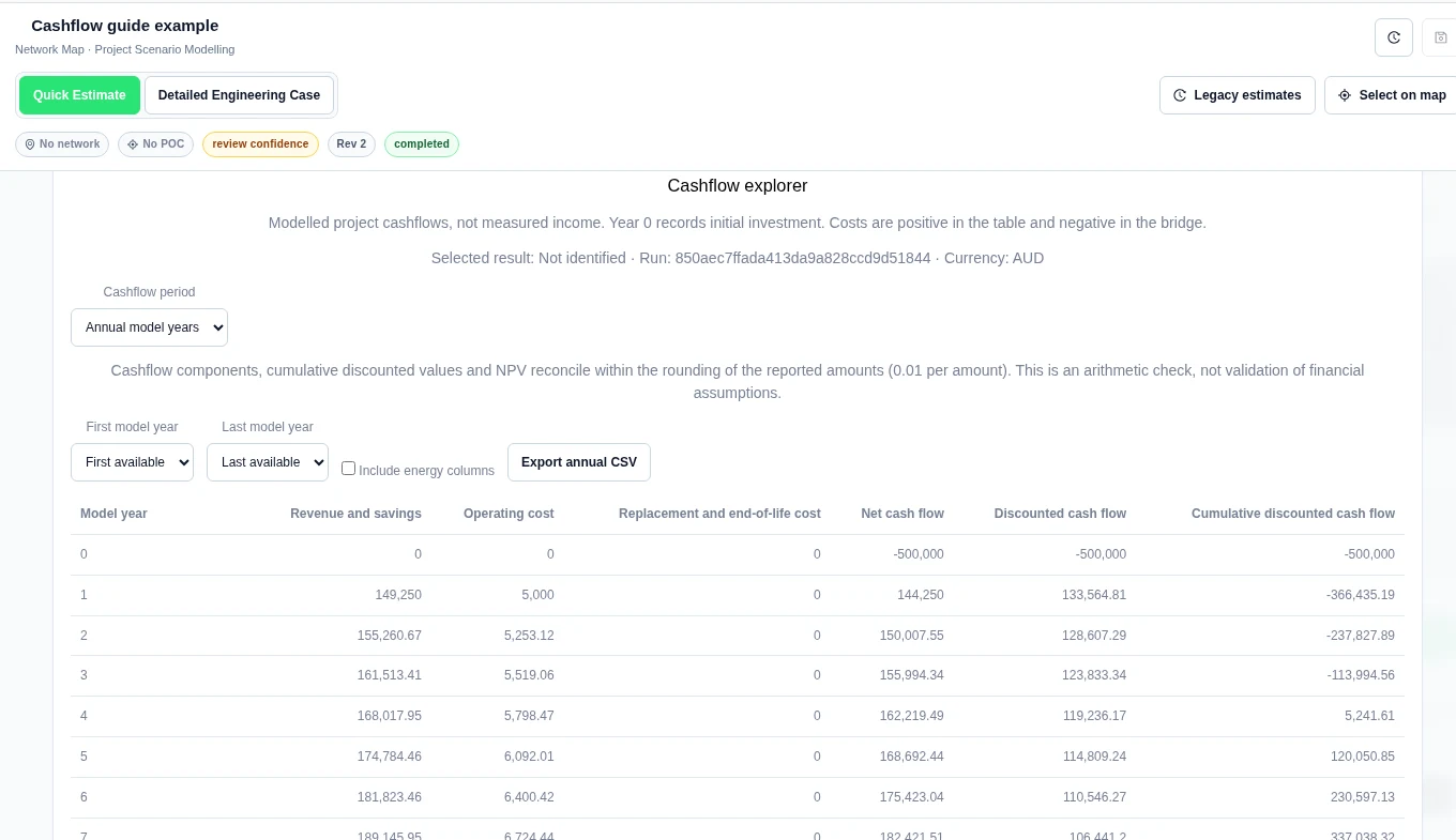
Run a saved case. Open Results, then Economics and Cashflow explorer. Keep Cashflow period on Annual model years. Check the recorded run and currency before reading amounts.
Year 0 records the initial investment. Later rows show revenue and savings, operating cost, replacement and end-of-life cost, net cash flow, discounted cash flow and the cumulative discounted balance. A dash means the result did not supply a value. It does not mean zero.
Choose years and inspect the bridge
Set First model year and Last model year to narrow the table and totals. The cumulative column keeps the original lifetime balance. It does not restart at the selected first year, and the closing balance is not a sum of that column.
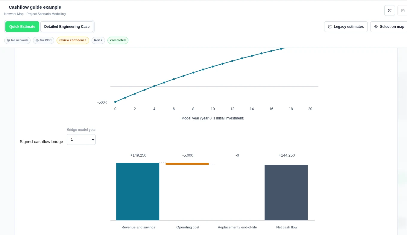
Choose a Bridge model year under Signed cashflow bridge. Costs appear as positive amounts in the table and negative bars in the bridge. The total is the sum of the signed components.
Worked example: a fresh Quick Estimate
This modelled example uses the unchanged new-case Quick Estimate assumptions: 500 kW solar, 500,000 AUD initial capex, 5,000 AUD first-year operating cost, a 20-year horizon and an 8% discount rate.
| Model year | Revenue and savings (AUD) | Operating cost (AUD) | Net cash flow (AUD) | Discounted cash flow (AUD) | Cumulative discounted cash flow (AUD) |
|---|---|---|---|---|---|
| 0 | 0 | 0 | −500,000 | −500,000 | −500,000 |
| 1 | 149,250 | 5,000 | 144,250 | 133,564.81 | −366,435.19 |
| 20 | 316,016.37 | 12,778.41 | 303,237.96 | 65,059.16 | 1,409,310.13 |
Replacement and end-of-life cost is 0 in these reported rows. Across years 0–20, the displayed discounted cash-flow total is 1,409,310.12 AUD. The reported closing balance is 1,409,310.13 AUD. The one-cent difference is within the rounding check. The check tests arithmetic, not whether the financial assumptions are suitable.
Export the displayed years
Choose Export annual CSV. The download includes the selected years, run ID, specification digest, recorded currency, missing-value notes and reconciliation status. It retains the precision supplied by the result. Select Include energy columns only when you also need the supplied energy values.
Read returns for an allocation
In Participant value allocation, select the recorded site and participant. Participant lifetime returns uses the selected allocation over all model years. Detail year and stream filters do not turn it into a partial-period investment return.
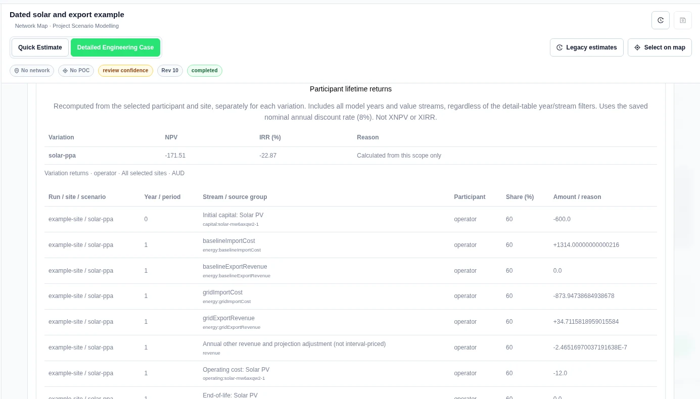
The whole example has 1,000 AUD initial capital cost, 791.27 AUD first-year revenue and savings, and 20 AUD first-year operating cost. At the recorded 8% discount rate, its full NPV is −285.86 AUD. These are modelled cash-flow outputs.
See Participant Allocation for the signed source flows. Use Saved Reports and Templates to choose a report's financial scope or build a batch by allocation.
Read dated cash flows
A completed Detailed Engineering Case can supply a dated ledger. Open Results → Economics → Cashflow explorer. Check the recorded run, currency and timezone. The ledger groups model accruals, not invoice or payment dates.
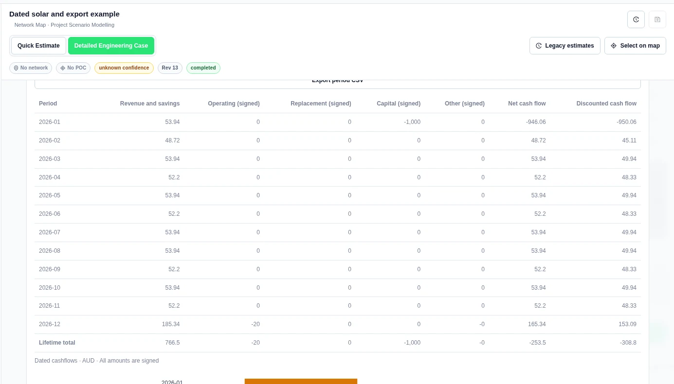
Choose Monthly
Set Cashflow period to Monthly. Each row uses the dated result. The product does not divide an annual total into twelve assumed months. Costs are signed in this dated table.
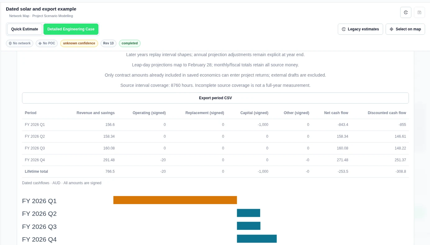
Choose Quarterly
Set Cashflow period to Quarterly. Choose Fiscal year starts to set the quarter boundaries. With January selected, the first quarter covers January to March.
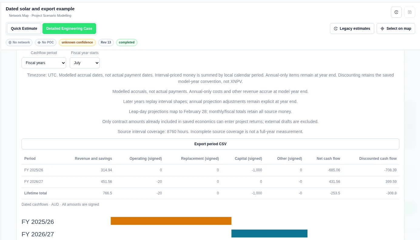
Choose Fiscal years and export
Set Cashflow period to Fiscal years. Select Fiscal year starts. Choose Export period CSV to download the selected period view. The file includes the run ID, currency, timezone, signed amounts and date basis. It retains source precision.
Worked example: dated solar and export
This is a separate example from the Quick Estimate above. We ran a one-year Detailed Engineering Case in AUD and UTC. It used 8,760 hourly load values of 1 kW for 2026. The 2 kW solar asset used a resource value of 1 pu for hours 10:00–15:00 UTC each day and 0 otherwise. The result reported PROFILE SOURCE provided, 4,380 kWh generation and 2,190 kWh onsite use.
The inputs were 1,000 AUD capital cost, 20 AUD annual operating cost, an 8% discount rate, 0.25 AUD/kWh import and 0.04 AUD/kWh export. No exact tariff was pinned. A saved 100 AUD/MWh export PPA replaced the scalar export credit. See Contract Settlement for its terms and settlement.
| Displayed period | Revenue (AUD) | Operating, signed (AUD) | Capital, signed (AUD) | Net cash flow (AUD) |
|---|---|---|---|---|
| 2026-01 | 53.94 | 0 | −1,000 | −946.06 |
| 2026-02 | 48.72 | 0 | 0 | 48.72 |
| 2026-12 | 185.34 | −20 | 0 | 165.34 |
| All twelve months | 766.50 | −20 | −1,000 | −253.50 |
With a January fiscal start, quarterly revenue is 156.60, 158.34, 160.08 and 291.48 AUD. With a July start, the fiscal-year rows are:
| Fiscal label | Modelled dates in this row | Revenue (AUD) | Net cash flow (AUD) | Discounted cash flow (AUD) |
|---|---|---|---|---|
| FY 2025/26 | January–June 2026 | 314.94 | −685.06 | −708.39 |
| FY 2026/27 | July–December 2026 | 451.56 | 431.56 | 399.59 |
All three period views reconcile to 766.50 AUD revenue, −253.50 AUD lifetime net cash flow and −308.80 AUD discounted cash flow. These are synthetic model outputs.
Related Guides
- Project Modelling
- DER Design
- Profiles and Inputs
- Network Tariffs
- Comparison and Reports
- Unit Revenue with Loss Factors
- Worked Examples


