Docs Menu
Engineering Plot Studio
Review study charts, compare numeric series, add reference bands, and download plotted data in Plot Studio.
Watch the Video: Plot Studio & Engineering Reports (1:10)
Open a plot
- Open Engineering Studies and complete a study, or open one from Study History.
- Check the study status, diagnostics and calculation basis in Study Results.
- Choose Plot Studio. Under Source, choose Plot template or Study chart.
- Select a template, or use Chart to select an output from the study.
Plots use the loaded study results. They do not run a new calculation. The available plots depend on the study, engine and returned data.
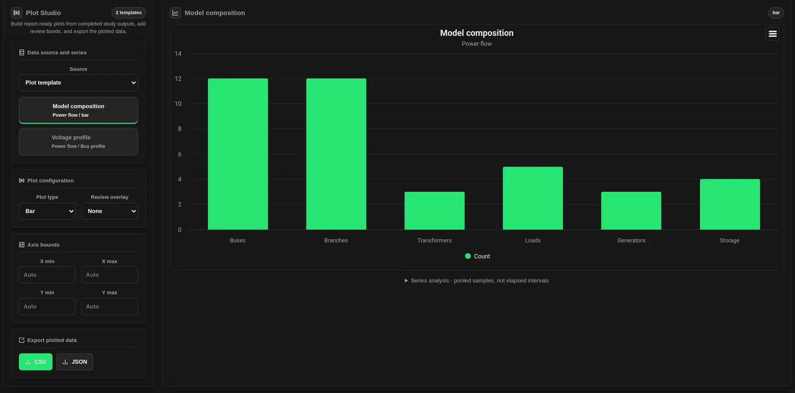
Study chart catalogue
Every returned study chart becomes a template. Engine-specific prefixes may appear in chart titles. Charts can be absent when a study did not produce the required results.
| Plot | What it shows | Review point |
|---|---|---|
| Model Composition | Counts of buses, branches, transformers, loads, generators and storage. | Model size, not data quality or solver success. |
| Voltage profiles and voltage cross-checks | Bus voltage in per unit, against bus names or IDs. | These are bus comparisons, not time traces. Check the engine and calculation basis. |
| Hosting Sweep Headroom | Remaining headroom against added generation steps. Voltage and loading series depend on the engine. | Read the binding constraint and status in the source table. Units may differ between series. |
| 24-Hour Loading Screen | Hourly load, generation and maximum loading. Some results also include minimum voltage. | These are study profile results, not live measurements. |
| Short-Circuit Fault Current Profile | Three-phase, line-line and line-ground fault-current series by bus, where returned. | Missing fault results are not zero current. Do not infer an equipment rating from a reference line. |
| Protection Coverage | Counts of covered branches, missing protection, coordination violations and breaker-duty violations. | This is a coverage summary, not a time-current coordination curve. |
Plot Connection Study tables
After running a Connection Study, open Results and choose Plot Studio. The selected alternatives supply a Stress-case selected-perspective NPV chart and a Stress-case engineering and value results table. The output names identify their alternatives.
- Under Source, choose Study table.
- Choose the alternative's table under Table.
- Choose a numeric X axis column.
- Select the numeric Y series to plot.
- Check the column units and review the original table before interpreting the relationship.
The table includes selected-perspective NPV and unserved energy in kWh, alongside stress-case and assessment labels. Use the plot with the original result table to compare alternatives and their assessment evidence. Automatic table templates need at least two columns with numeric values. Supplied study charts remain available under Study chart.
Choose series and chart type
Use Plot type to choose the chart format.
- Time series draws a line. Its horizontal labels can be hours, buses or other categories; check the labels for the axis meaning.
- Scatter uses numeric X values. If a category is not numeric, its row position is used instead.
- Bar draws vertical columns.
- Use Study chart to change the type of a supplied chart. Templates provide preset views.
Review overlays
Choose Review overlay to add a visual guide. The initial choice comes from the plot name, not from a check of its units or the study limits.
| Overlay | Reference shown | Use with care |
|---|---|---|
| None | No extra guide. | Use when units or limits are uncertain. |
| Voltage band | Band from 0.95 to 1.05; review lines at 0.9 and 1.1. | For per-unit voltage only. These fixed values do not track your study assumptions. |
| Thermal limits | Warning band from 80 to 100; lines at 80 and 100. | For loading percentages, not MW or amperes. |
| Fault duty | A breaker-duty reference line. | Do not rely on this overlay without a verified rating. See the warning below. |
| Frequency band | Band from 49.85 to 50.15; review lines at 49 and 51. | A fixed 50 Hz reference. It does not create a frequency-response result. |
| P/Q reference | X and Y zero lines, plus Y references at +0.395 and −0.395. | Not an equipment capability envelope. Check axes and scaling. |
| Custom reference | A horizontal line at Custom reference value. | Enter a numeric value in the plotted Y units. A blank or invalid value adds no line. |
Axes, chart interaction and statistics
Under Axis bounds, set X min, X max, Y min and Y max. Leave a field blank for Auto. On categorical line or bar plots, X bounds refer to category positions. Hover for values. Drag across the chart to zoom. Use legend entries to hide or show series.
- Samples: the total number of numeric Y values across the supplied series.
- Min / Max: the smallest and largest of those values.
- Mean / Final: the mean across those values, and the last numeric value of the last series.
- Settling Index: a sample index based on proximity to that final value, expressed as an index rather than elapsed time.
Statistics combine series in series order. They do not become separate per-series statistics when you hide a legend entry or zoom. Use one compatible series for response analysis. The settling band is the larger of 5% of initial-to-final change, 1% of the final magnitude, and a small numerical floor.
Plot Book
Plot Book shows up to eight generated templates, with study charts before eligible table plots. The plot count can be larger than the number displayed. Select other templates in the source list. Book panels use their own default types, overlays and automatic axes; they do not mirror all active-plot changes.
Inspect tables and map results
Use the study tabs to inspect the source tables and geographic results.
- Open Study Results, then choose a table under Result Tables. Paged tables use Previous page and Next page, with up to 100 rows per page.
- Use Result Charts to review supplied charts and return to Plot Studio.
- Open Result Layers. Use the eye control and opacity slider for each layer. Auto-fit controls fitting when supported by the map action.
- Choose Add to Map or Update Map. Added to Map indicates the current results are already shown. Use Remove from Map to clear them.
Map layers are separate from chart overlays. A chart can exist without geographic results. If a layer exceeds the 50,000-feature browser limit, zoom to a smaller map area and try again.
Export a plot
- Under Export plotted data, choose CSV for the active plot's index, category and Y-series values.
- Choose JSON for the active plot object and its series. This download is not a complete saved workspace. Axis bounds and the custom reference entry are not included in this file.
- The chart menu provides chart export and data actions. These are separate from the studio's CSV and JSON buttons.
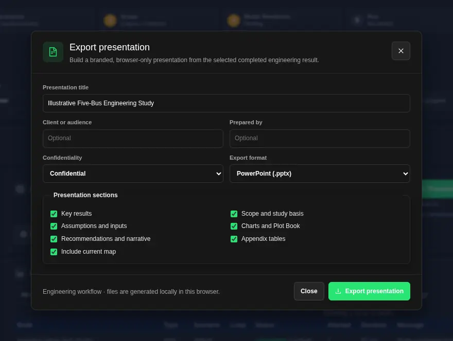
- For a report, return to Study Results and choose Presentation when enabled. The current study's plot state can feed the presentation. Exports & Handoffs is a separate completed-study package workflow.
The studio CSV is not a full result-table export. Use JSON when you need each scatter point's X and Y values.
When a plot is unavailable
- No result loaded: complete or open a study.
- No chart available: use Open Results when offered, then read diagnostics and tables.
- Empty or missing series: check study status and source data. Do not replace missing values with assumed zeros.
- Missing map action: the study may have no visible geographic result layers.
- Presentation disabled: check that the study is completed, its current results have loaded, and the result is eligible.
Charts in Workflow Runs
Plot nodes in Projects and Flows make their own charts. To open one, choose Runs, select a completed run, then choose View result on a plot node. The chart shows under Charts.
- Charts follow the app theme. In the dark theme, the chart, grid and labels are dark too.
- Each chart draws in once when it opens. This is a display animation in the app. It is not a playback of the simulation. If your device asks for reduced motion, the chart shows at once with no animation. Downloaded chart images do not move.
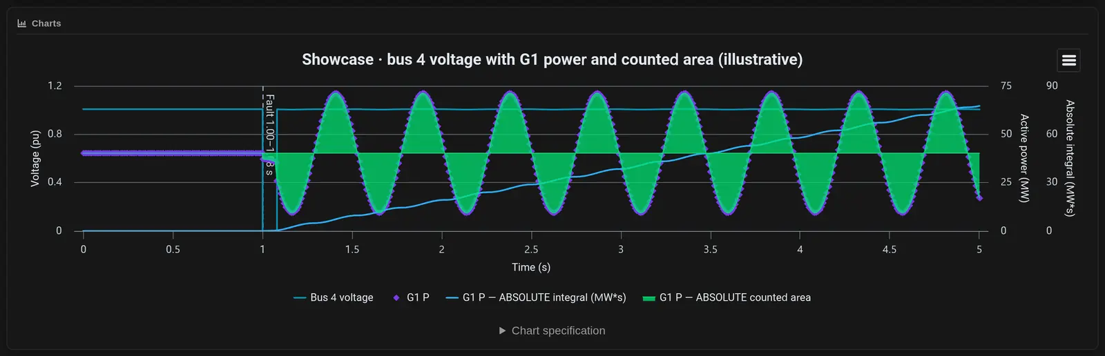
The examples below use simulated results from a five-bus model.
Mixed axes
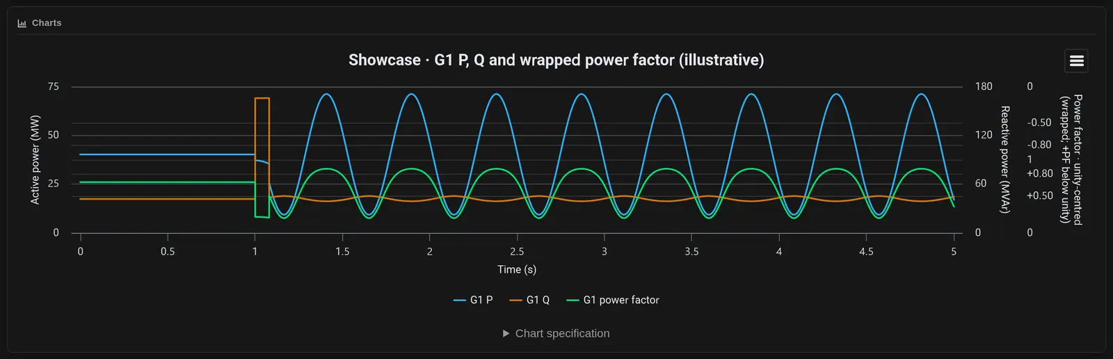
A plot can put series on a left axis and a right axis. Use this when quantities have different units, such as bus voltage in per unit and generator power in MW. In the plot node settings, find Pages and subplots and tick Use pages and subplots. For each series in a subplot, set Axis to Left (primary) or Right (secondary). Enter a Left axis title and a Right axis title. Always read the axis title before you compare two lines.
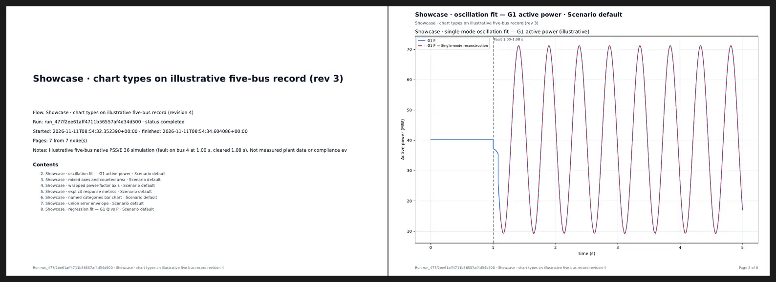
Oscillation fit
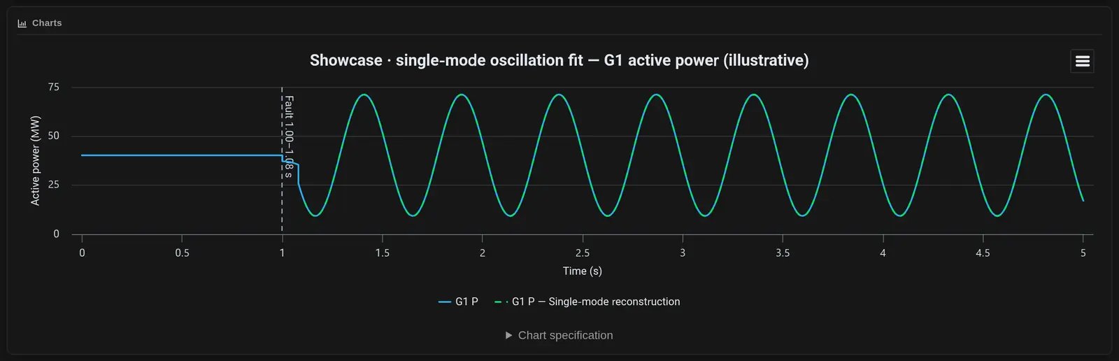
In the plot node settings, open Advanced signal analysis. Turn on Reconstructed dominant oscillation. Set the start and end time in seconds, and the frequency range to search. The fit draws one damped or growing sine wave plus an offset over the signal.
Check R², the residuals, the sample coverage and any warnings before you read the damping. The fit describes the plotted signal over the selected window.
Wrapped power factor axis
Under Reference lines, envelopes and power factor, choose Add power factor channel and pick the P and Q columns. Then set Power-factor axis presentation to Unity-centred wrapped axis. This axis keeps values near 1.0 easy to read. The default is Signed linear (-1 to 1; existing default).
Regression fit
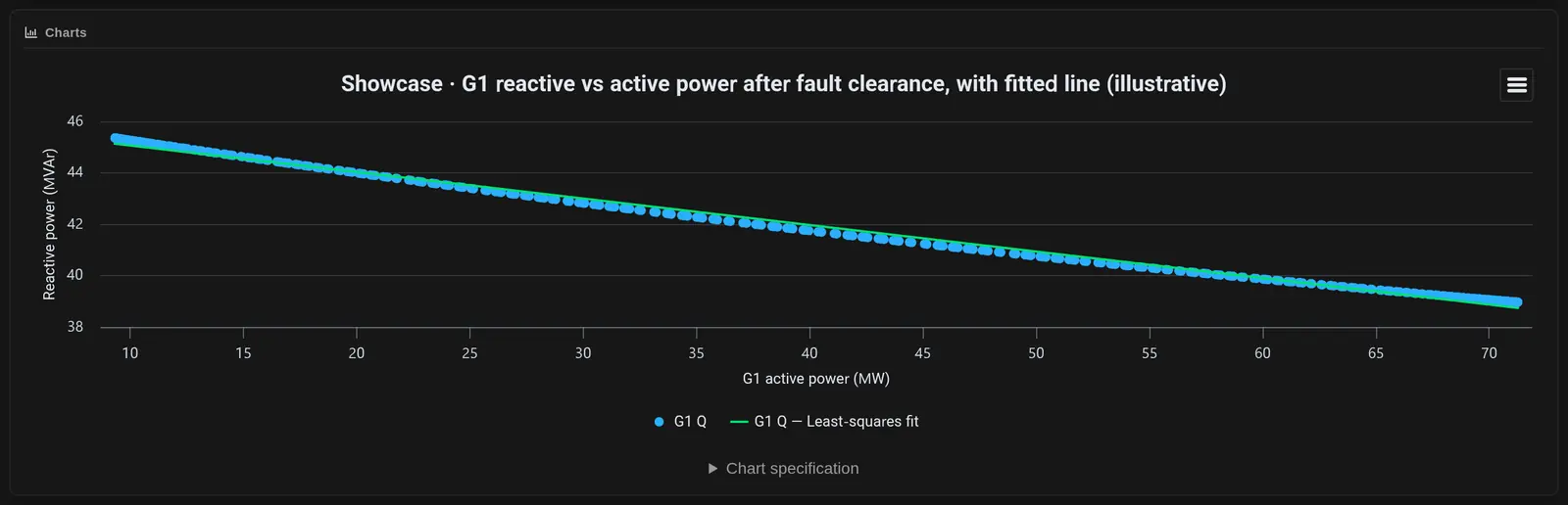
In Advanced signal analysis, turn on Least-squares regression. It fits Y against X over the selected points. You can set an X range and the units. The chart shows the points and the fitted line.
Response metrics
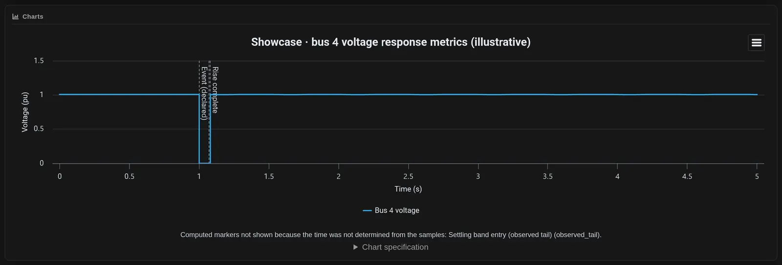
Under Response measurements, set the event time and the other values. The chart marks the points it finds on the trace, such as the declared event and rise complete. If a time cannot be found from the samples, the chart lists it under the plot and does not draw that marker.
Benchmark Two Result Records
Benchmark two results is in Vendor run package, separate from the Plot Studio chart controls. Select the reference and candidate files, then check channel names, units and sign conventions. Record any time shift.
The comparison uses the common time window and interpolates the candidate onto the reference time points. It reports Max error, RMS error and Mean error for each channel. With no band set, it reports metrics only, with no pass or fail. Keep the source of any acceptance band with your study notes.
Record the reference source, selected channels and comparison window with the benchmark results.
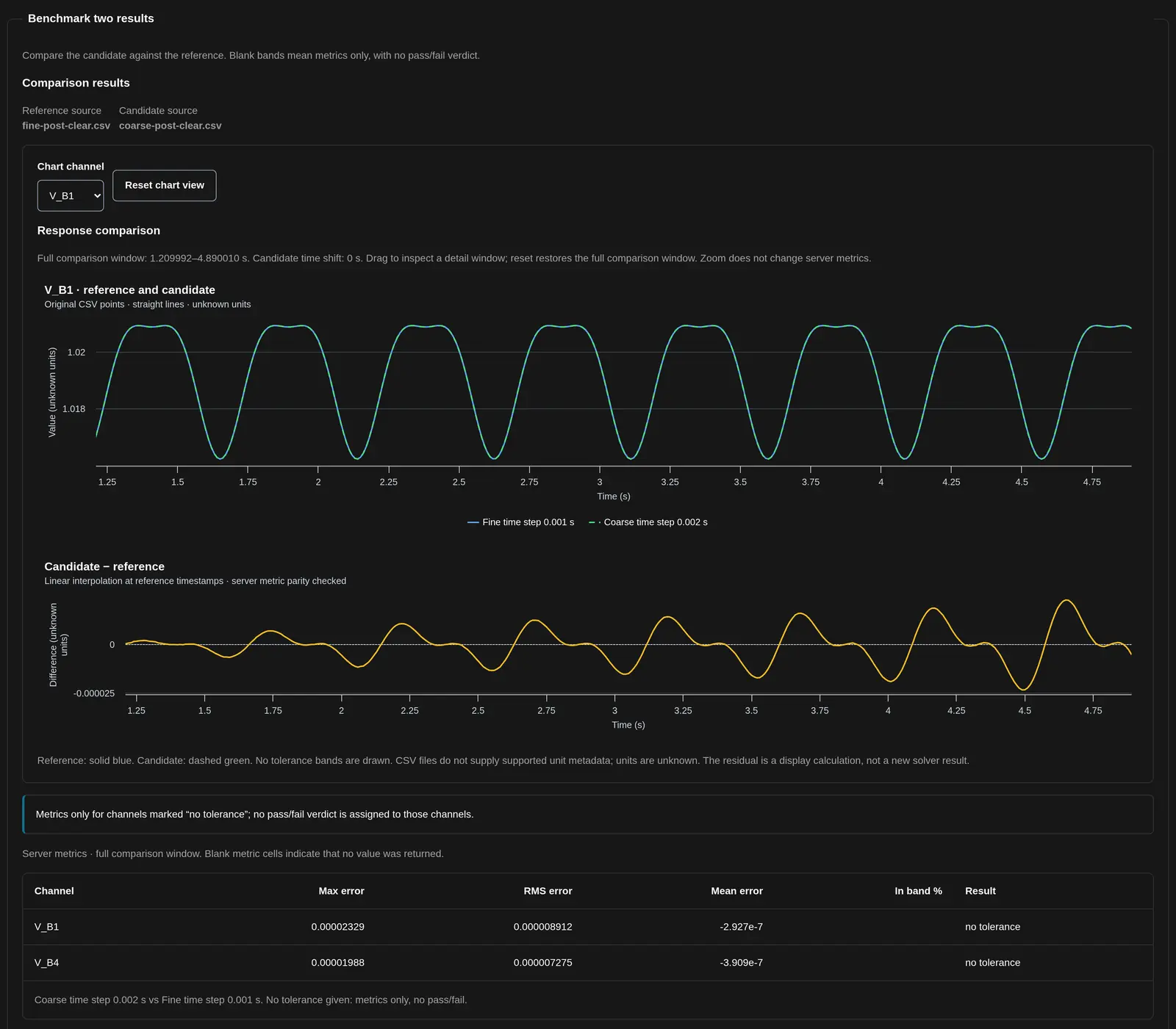
For step-by-step use, see Benchmark two result sets.
Choose the Report Output
- Workflow run plot report: a PDF or HTML collection of available completed-run charts, from the workflow Runs view.
- Study Presentation: a PowerPoint or PDF summary; large result sets can be shortened.
- Export plotted data: CSV or JSON for the active plot, not a full electrical-model interchange package.
Open the output before sharing it. Check the case, legible units, included plots and omitted material. Retain the model revision and run identity alongside the report.