

Docs Menu
DER Design
Configure solar, wind, hydro, biomass, storage, and load changes at the case's point of connection.
Add and manage assets
- Open DER Design.
- Choose Asset type.
- Select Add Asset.
- Enter Asset name under Identity & connection.
- Complete Sizing & operation.
- Complete Costs & lifecycle.
A new case already contains one Solar PV asset. You can add several assets, including several of the same type. The asset count appears above the cards. Use the delete button on an asset card to remove that asset. Keep at least one DER or load-adjustment asset to run the case.
All cards use the point of connection selected in Map Scope & Connection. There is no separate connection-point selector on each card. Each card shows its type, connection-point name, and source.
Common identity and connection fields
| Field | Default | Use |
|---|---|---|
| Asset name | The asset type name. | Use a unique, useful name. It appears in asset selectors and sweep targets. |
| Power factor | 0.95 | Shown for generation and storage, but not load adjustment. Generator power factor informs reactive-power modelling. Do not treat this field alone as a verified inverter-control model. |
Solar PV
| Field | Default | Meaning |
|---|---|---|
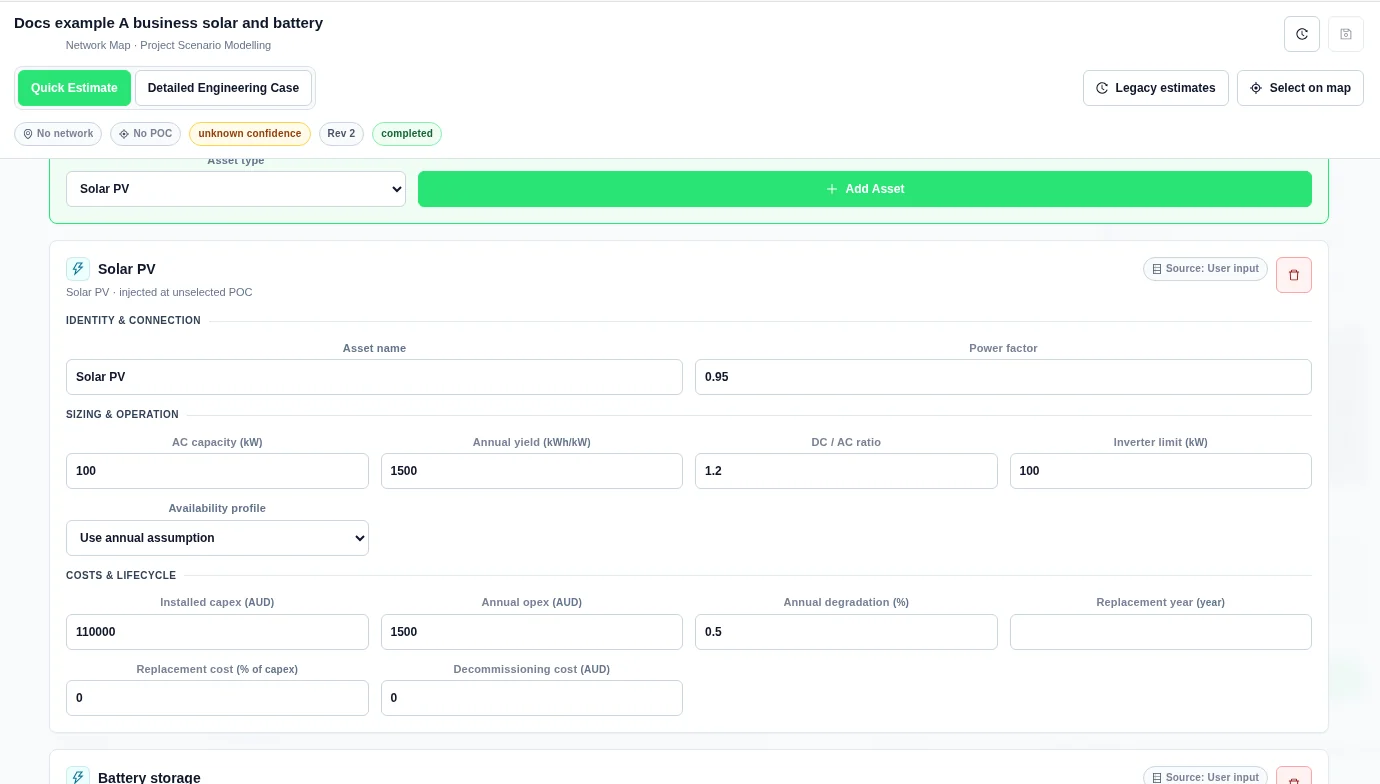
| AC capacity | 500 kW | Installed AC generation capacity. |
| Annual yield | 1,500 kWh/kW | Annual energy assumption per kW of capacity. |
| DC / AC ratio | 1.2 | Ratio of DC array capacity to AC capacity. |
| Inverter limit | 500 kW | AC inverter output limit. |
| Availability profile | Use annual assumption | Choose an attached resource-availability or generation profile for the chronological shape. Supply normalized pu values from 0 to 1. |
Detailed solar dispatch uses the availability shape and DC/AC sizing, with AC capacity and inverter limits. A positive Annual yield scales the shape toward the annual energy target, subject to output limits. A generic solar shape needs review. Attach a suitable interval resource profile for a detailed conclusion.
Solar input example
Wind
| Field | Default | Meaning |
|---|---|---|
| Rated capacity | 500 kW | Installed generator capacity. |
| Annual yield | 2,200 kWh/kW | Annual energy assumption per kW. |
| Derating | 5% | Reduction applied to generation output. |
| Availability profile | Use annual assumption | Choose an attached normalized availability or generation shape. A positive Annual yield scales the shape toward the annual energy target before derating, subject to capacity limits. The card does not calculate wind resource from site coordinates. |
Hydro
| Field | Default | Meaning |
|---|---|---|
| Generator capacity | 500 kW | Installed generator capacity. |
| Operating mode | Run of river | Choose Run of river or Dispatchable. Run-of-river output follows resource availability. Dispatchable hydro can respond within its operating assumptions. |
| Annual energy budget | 2,000,000 kWh | Energy budget for the hydro asset. |
| Minimum output | 0% | Minimum operating output as a percentage of capacity. |
| Availability profile | Use annual assumption | Select an attached availability or generation shape. Confirm that it represents the available hydro resource. |
Biomass
| Field | Default | Meaning |
|---|---|---|
| Generator capacity | 500 kW | Installed generator capacity. |
| Fuel / marginal cost | 55 per MWh | Variable generation cost in the case currency per MWh. |
| Minimum output | 25% | Minimum operating output as a percentage of capacity. |
| Ramp rate | 10%/min | Requested change in output per minute. Confirm the operating assumption against equipment data. |
| Availability | 90% | Availability multiplier. |
| Availability profile | Use annual assumption | Select an attached availability or generation shape when available. |
Biomass is dispatchable in the detailed model. The availability, minimum-output, fuel-cost, and ramp assumptions affect its operating model. This is not a plant control-system simulation.
Battery storage
| Field | Default | Meaning |
|---|---|---|
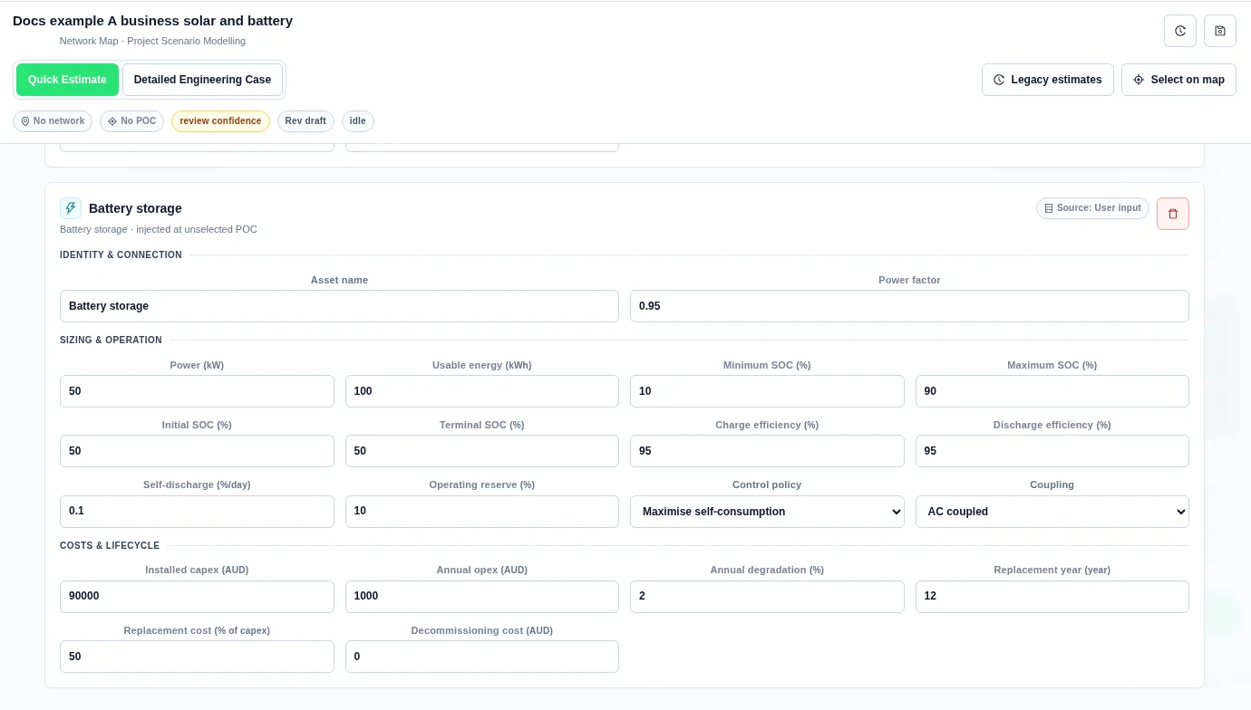
| Power | 100 kW | Charge and discharge power rating. |
| Usable energy | 200 kWh | Energy capacity entered for the model. The state-of-charge window and reserve further constrain operation. |
| Minimum SOC | 10% | Lower state-of-charge boundary. |
| Maximum SOC | 90% | Upper state-of-charge boundary. |
| Initial SOC | 50% | State of charge at the start of the dispatch period. |
| Terminal SOC | 50% | State-of-charge target at the end of the period. Review terminal-state diagnostics in detailed results. |
| Charge efficiency | 95% | Efficiency when energy enters storage. |
| Discharge efficiency | 95% | Efficiency when stored energy is delivered. |
| Self-discharge | 0.1%/day | Daily stored-energy loss assumption. |
| Operating reserve | 10% | Capacity reserved from ordinary dispatch. |
| Control policy | Maximise self-consumption | Select the dispatch objective described below. |
| Coupling | AC coupled | Choose AC coupled or DC coupled. DC coupling requires follow-on review of inverter clipping and DC-bus losses. |
Storage control policies
| Policy | Use |
|---|---|
| Maximise self-consumption | Store excess generation and discharge against site demand. |
| Peak shaving | Use storage to reduce peaks in site import. |
| Tariff arbitrage | Use price differences to guide charging and discharging. Confirm the price assumptions in Value & Finance. |
| Network support | Dispatch storage against the modelled network-support target and limits. |
Storage validation
- Power and Usable energy must be greater than zero.
- Maximum SOC must exceed Minimum SOC.
- Initial SOC and a supplied Terminal SOC must be inside the SOC window.
- Operating reserve must not exceed the difference between maximum and minimum SOC.
- Charge and discharge efficiencies must be greater than zero and no greater than 100%.
If the server reports initialSocPercent must be inside the SOC operating window, correct Initial SOC or the SOC limits. Apply the same rule to a terminal-SOC message. For reservePercent exceeds the usable SOC window, reduce the reserve or revise the SOC limits.
Battery input example
Load adjustment
| Field | Default | Meaning |
|---|---|---|
| Adjustment type | New demand | Choose New demand, Load growth, or Demand reduction. Demand reduction subtracts energy from baseline load; the other choices add demand. |
| Peak demand change | 250 kW | Peak demand-change assumption. |
| Annual energy change | 500,000 kWh | Annual energy added or removed. Enter its magnitude; the adjustment type determines the direction. |
| Annual growth | 0% | Annual growth assumption for the adjustment. |
| Availability profile | Use annual assumption | Choose an attached availability or generation profile to shape the adjustment over time. |
Provide a positive peak demand change or annual energy change. Prefer a confirmed annual energy change instead of relying on a peak-only estimate. Use the load adjustment to model the demand change, and enter the applicable connection limits separately.
Costs & lifecycle
Every asset card includes these fields. Values are asset-specific, not a single shared project budget.
| Field | Default | Meaning |
|---|---|---|
| Installed capex | 0 in the case currency | Initial installed capital cost. |
| Annual opex | 0 in the case currency per year | Annual fixed operating cost. |
| Annual degradation | 2% for storage; 0.5% for other new asset cards | Annual degradation assumption. Confirm its relevance to the asset type and calculation mode. |
| Replacement year | Blank | Year when a replacement cost is incurred. Leave it blank when no replacement is specified. |
| Replacement cost | 0% of capex | Replacement cost as a percentage of initial capex. |
| Decommissioning cost | 0 in the case currency | End-of-life cost assumption. |
Enter explicit values for known costs. A blank numeric input is not evidence that a cost is zero. See Value and Finance for financial methods and lifecycle treatment.
Link profiles and options
- Upload the relevant files in Demand & Resource Profiles.
- Return to each asset card.
- Select its Availability profile where that control is present.
- Open Options to sweep generator capacity, storage power, storage energy, or storage reserve.
- Check that each sweep targets a compatible asset.
The availability selector offers attached Resource availability and Existing generation profiles. Choose data that matches the intended asset. Storage has its own operating controls rather than an availability selector in this workbench.
Screening and explicit performance bindings
Asset performance and charging provides typed screening attachments. An unbound screening check does not change case totals. An explicit battery capacity binding can affect saved runs. Operating-window library items can also create a load profile for a Load adjustment asset.
See Asset Screening for real input and result examples. For timed operating bounds on battery equipment, see Dispatch Calendars and Sizing.
See Shared Library for target selection, saved version pins, profile coverage and the save-and-rerun steps.


