

Docs Menu
Asset Screening
Check supplied charging plans, flexible-load windows and genset assumptions before using them in a study.
Add and assess an attachment
- Open Project Modelling → Design → Asset performance and charging.
- Choose Attachment type, then New attachment. Give it a unique Attachment ID, a Name and a Source / evidence reference.
- Enter your own data. Keep missing values blank. Use dated windows with explicit UTC offsets and an IANA timezone.
- Finish the typed editor. Select Validate and assess.
- Review Screening estimates, units, missing-data reasons and Supplied-limit checks.
- Select Apply to draft case, then Save case revision to retain the attachments.
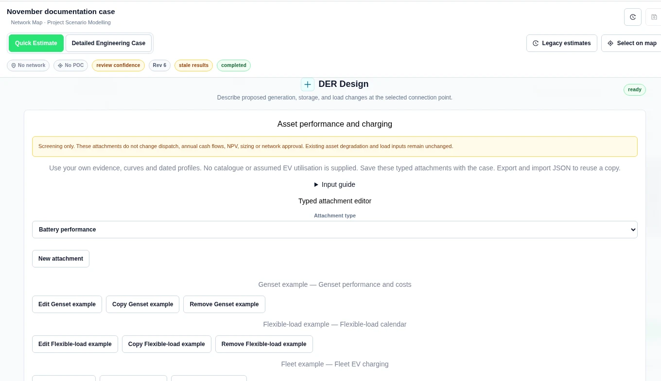
Advanced JSON and reuse provides Asset screening JSON, Import JSON (up to 1 MiB) and Export draft JSON. Import replaces the screening draft, not the saved case. Finish or cancel a typed edit before importing. Use Input guide and Load field schema for the JSON fields.
Check a genset at steady output
Choose Genset performance and costs. Supply Rated electrical power (kW), Assessment output (kW), Running hours, a Part-load curve and optional Running costs. State the thermal basis and curve source. Choose heat rate or efficiency; do not mix their units.
Worked example
We used 100 kW rated output, 75 kW assessment output and 2 running hours. The heat-rate curve used 4 kWh_th/kWh_e at load fraction 0.5 and 3 at fraction 1. The stated basis was net electrical output and lower heating value. Costs were AUD: fuel 0.1 per kWh thermal, variable 0.02 per kWh electrical and 3 per running hour.
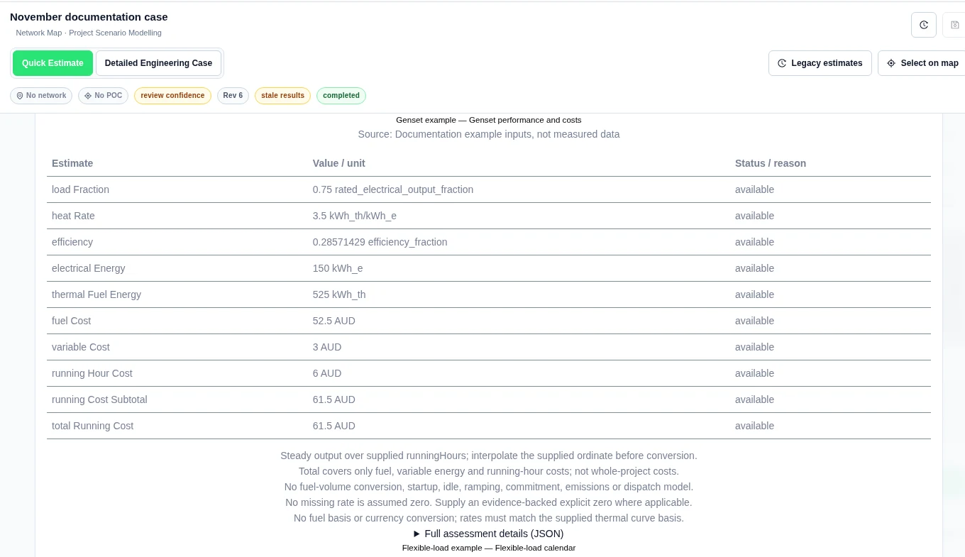
| Result | Product value |
|---|---|
| Load fraction | 0.75 |
| Heat rate | 3.5 kWh_th/kWh_e |
| Electrical energy | 150 kWh_e |
| Thermal energy | 525 kWh_th |
| Fuel / variable / hourly cost | 52.5 / 3 / 6 AUD |
| Total assessed cost | 61.5 AUD |
This is steady-output screening. It has no idle fuel, startup, commitment or dispatch model. The curve is not extrapolated. Missing cost rates are not zero.
Check flexible-load capacity
Choose Flexible-load calendar. For each Energy windows row, enter start, end, Required energy (kWh) and Maximum power (kW). Use ordered, non-overlapping windows.
Worked example
For 1 November 2026, 10:00–12:00 UTC, we entered 15 kWh required and 10 kW maximum power. The product returned 20 kWh maximum energy, 0 kWh shortfall and within supplied limits.
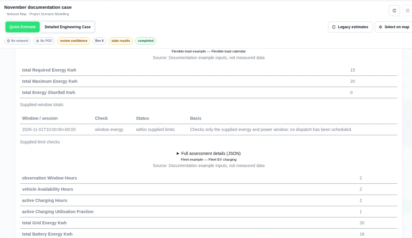
This check does not schedule the load. Review equipment and site connection limits when building a schedule.
Check fleet charging
Choose Fleet EV charging. Enter fleet and charger counts, charger input power and charging efficiency. Add Vehicle sessions with arrival/departure times, battery capacity, arrival SOC, target SOC and maximum vehicle input power. Supply the Charging plan; the tool does not create one.
Worked example
Our input had 2 vehicles and 1 charger rated 10 kW, with efficiency 0.9. One vehicle session ran on 1 November 2026 from 10:00–12:00 UTC. Its battery was 50 kWh, arrival SOC 20%, target SOC 56% and maximum vehicle charge power 11 kW. The supplied plan charged at 10 kW for the whole two hours.
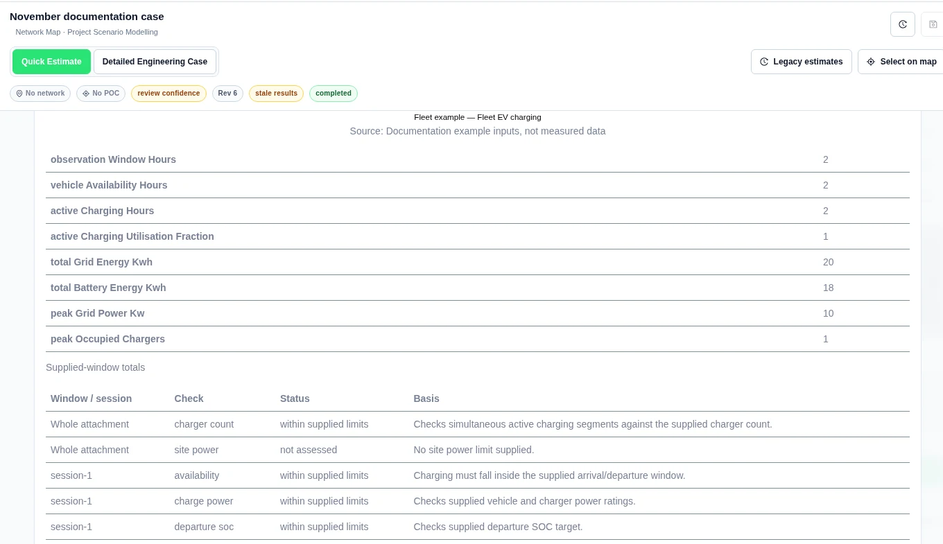
| Result | Product value |
|---|---|
| Grid energy | 20 kWh |
| Battery energy | 18 kWh |
| Peak grid power | 10 kW |
| Peak occupied chargers | 1 |
| Active charging utilisation fraction | 1 |
| Departure SOC check | Within supplied limits |
No site power limit was supplied, so that check was not assessed. This is not zero site demand. Missing charging-plan data means unknown, not idle. There is no vehicle driving model.
Check on-demand charging
Choose On-demand charging. Enter chargers and efficiency, then Utilisation windows with session count, occupied charger-hours, grid energy and sold energy. Add explicit currency under Charger costs and sales rates. Supply peak grid power and a site limit if you want the corresponding power checks.
Worked example
We used 2 chargers at 10 kW each and efficiency 0.9. The same two-hour UTC window had 3 sessions, 2 occupied charger-hours, 20 kWh grid energy and 18 kWh sold. Rates in AUD were 0.2 per grid kWh, 0.5 per sold kWh and 1 per session. Each charger cost 1,000; installation cost 500; fixed annual operating cost was 100.
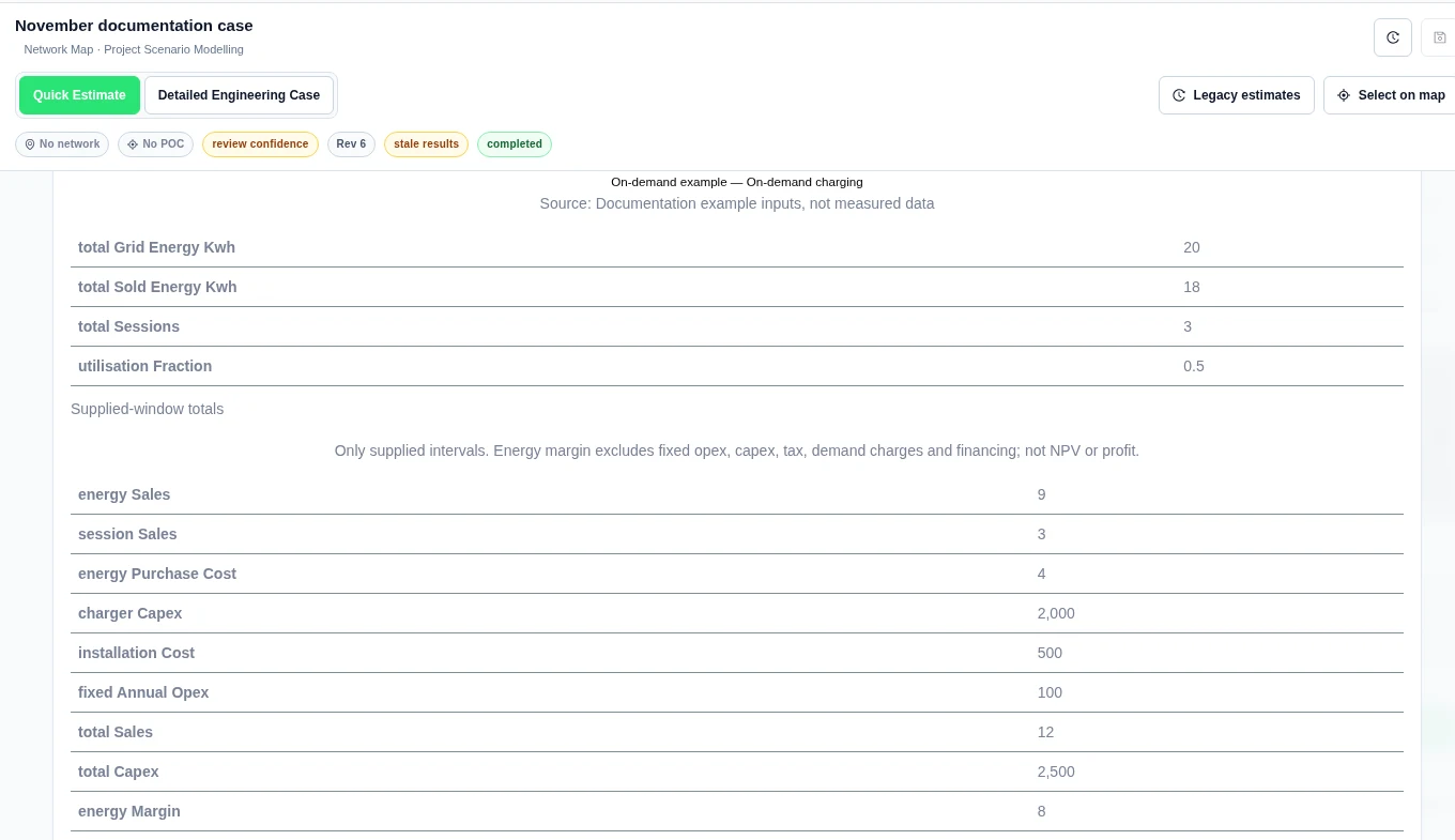
| Result | Product value |
|---|---|
| Utilisation fraction | 0.5 |
| Energy sales / session sales | 9 / 3 AUD |
| Total sales | 12 AUD |
| Energy purchase cost | 4 AUD |
| Energy margin | 8 AUD |
| Capex | 2,500 AUD |
Use a bound battery curve in a run
- In Profiles → Shared input library, apply the battery equipment item to the case.
- Select the performance item and its exact Version. Set Target case asset to that battery and choose Apply pinned item to case.
- Review Design, save a case revision and run the case.
- Open Results → Energy → Applied asset curves. Expand the binding to inspect its source pin, applied-input digest and year-by-year values.
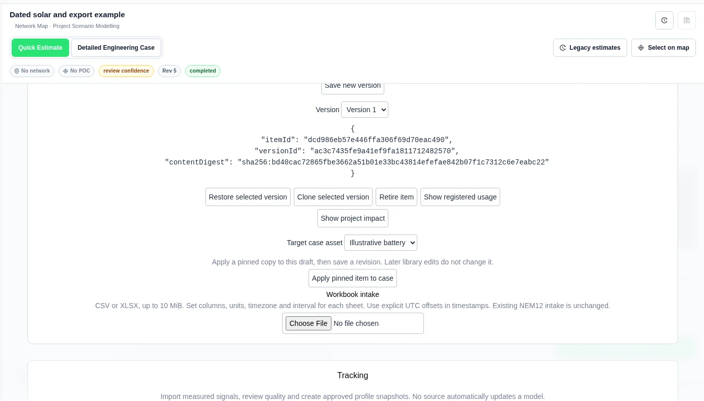
Worked example: a two-year capacity curve
Our synthetic battery had 20 kW power and 40 kWh capacity. The age curve supplied retained fraction 1 at age 0 and 0.9 at age 1. We used age 0 and a two-year horizon. The completed Quick Estimate showed:
| Model year | Capacity | Retention |
|---|---|---|
| 1 | 40 kWh | 1 retained_fraction |
| 2 | 36 kWh | 0.9 retained_fraction |
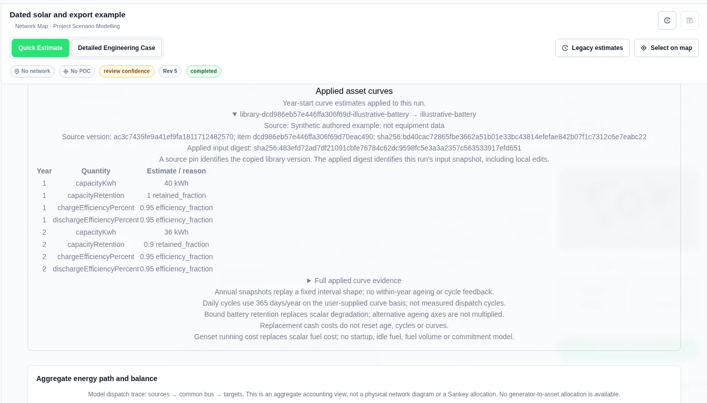
These are user-supplied performance estimates. Year-start snapshots replay a fixed interval shape. There is no within-year ageing or cycle feedback. Daily cycles use 365 days per year on the supplied basis, not measured dispatch cycles. Bound battery retention replaces scalar degradation; alternative ageing axes are not multiplied. Replacement cash costs do not reset age, cycles or curves.
Genset running costs use an explicit compatible equipment binding. They replace scalar fuel cost. They do not model startup, idle fuel, fuel volume or unit commitment. Bound solar and wind primary and balance-of-system curves multiply and replace scalar degradation. Optional weather conversion needs the complete supplied inputs described below.
Convert supplied weather to solar and wind power
Use your own complete weather year and explicit equipment models. The product does not fetch weather, infer missing channels or predict future weather. Results are estimated generation profiles.
Bind the model to the equipment
- Add solar or wind equipment in Design. Keep nameplate capacity, AC/DC sizing and costs explicit.
- In Profiles → Shared input library, save an asset_types.solar or asset_types.wind attachment. Include initial age and both primary and balance-of-system retention curves.
- Select the exact Version and Target case asset, then Apply pinned item to case.
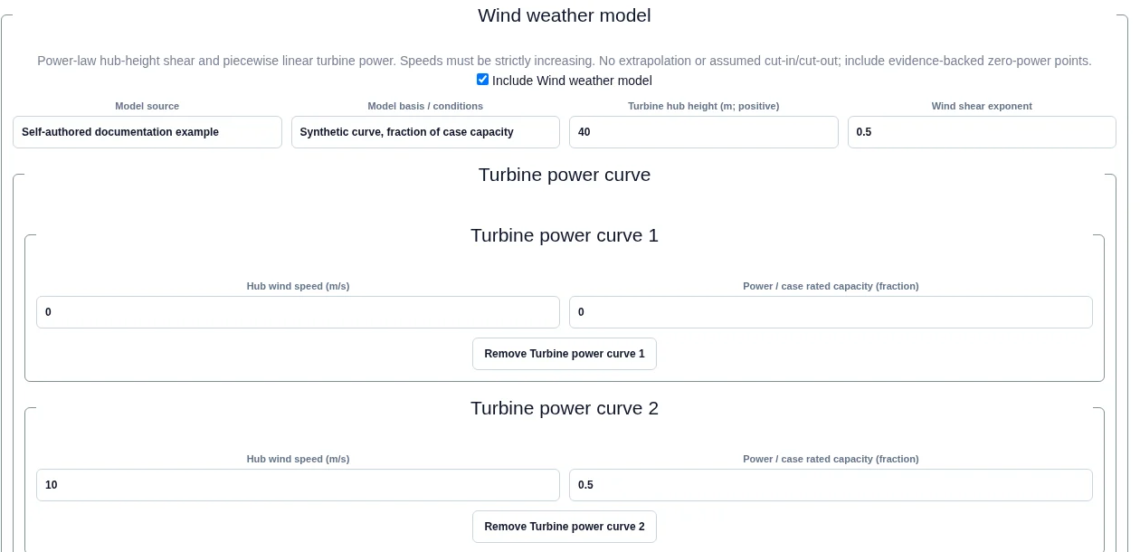
- In Design → Asset performance and charging, review the attachment. Solar weather model needs tilt, azimuth, albedo, the module temperature coefficient, reference temperature and irradiance, and inverter efficiency. Wind weather model needs hub height, shear exponent and a turbine power curve.
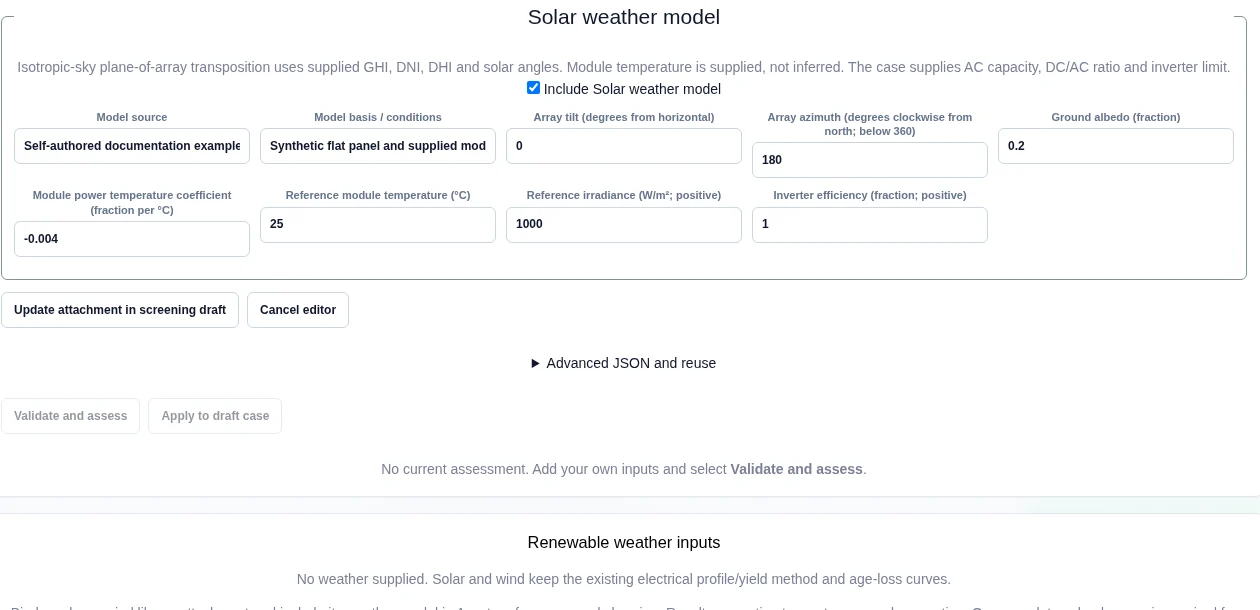
If you edit an attachment, select Update attachment in screening draft, then Validate and assess and Apply to draft case. Local edits do not change the source library version.
Import and apply a full calendar year
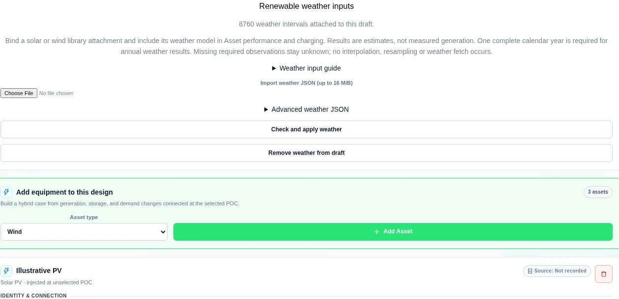
- Open Design → Renewable weather inputs → Weather input guide.
- Use Import weather JSON (up to 16 MiB) or Advanced weather JSON. Import changes the review draft only.
- Supply
source,intervalMinutesand ordered, unique interval-starttimestampswith explicit UTC offsets. Every channel must match the timestamp count. Allowed intervals are 5, 10, 15, 30 or 60 minutes. - Review the input, then select Check and apply weather. Save a case revision and run.
| Asset | Required weather channels |
|---|---|
| Solar | ghiWm2, dniWm2, dhiWm2 in W/m²; solarZenithDeg, solarAzimuthDeg; moduleTemperatureC. Azimuth is clockwise from north and below 360°. |
| Wind | windSpeedMps in m/s and positive windReferenceHeightM in metres. |
Check the saved evidence
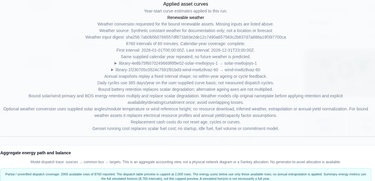
Open Results → Energy → Applied asset curves. Check Weather source, Weather input digest, first and last intervals, calendar-year coverage and the asset bindings. Expand a binding to inspect its exact library pin, applied-input digest and year-start retention.
Worked example: weather-to-generation conversion
We used one full synthetic 2026 weather year built for this guide. The sun follows a simple clear-sky path for a southern-hemisphere site, with a repeating cloud factor. Wind speed varies by season and through the day. The case has a 2 kW solar asset, a 2 kW wind asset and a 2 kW / 4 kWh battery, with an 8,760 kWh annual load.
- Solar: hourly GHI, DNI and DHI follow the sun path and are 0 W/m² at night (4,381 of 8,760 hours). Solar angles come from the same path. Module temperature rises with irradiance. The flat-panel model uses DC/AC ratio 1, reference irradiance 1,000 W/m², reference temperature 25°C, coefficient −0.004 per °C and inverter efficiency 1.
- Wind: hourly speed at 10 m varies between 0 and 9.5 m/s. Hub height is 40 m and the shear exponent is 0.5, so hub speed is twice the supplied speed. The supplied curve is 0 fraction at 0 m/s, 0.5 at 10 m/s and 1 at 20 m/s. Wind derating is 0%.
- Both assets start at age 0. Primary and BOS curves retain fraction 1 throughout this conversion-only example. No age loss is assumed.
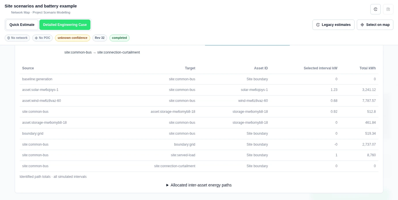
Completed Detailed run 038f5d4bf6d1443c8532e73a3b48334e showed 3,241.12 kWh from solar and 7,787.57 kWh from wind, a total of 11,028.68 kWh. Solar output is zero at night and peaks below the 2 kW AC limit, so Clipped energy is 0 kWh in this example. The site imported 519.34 kWh and exported 2,737.07 kWh. Self-sufficiency was 94.07%. The product’s asset-path totals cover all 8,760 hours, not just the 2,000-row browser preview, and the energy balance closes.
Model formulas and limits
Solar plane-of-array irradiance is direct normal irradiance × positive incidence cosine, plus DHI × (1 + cos tilt)/2, plus GHI × albedo × (1 − cos tilt)/2. Direct beam is zero below the horizon. Incidence uses the supplied solar angles and array orientation.
DC power is case AC capacity × DC/AC ratio × plane-of-array irradiance / reference irradiance × max(0, 1 + temperature coefficient × (module temperature − reference temperature)). Inverter efficiency applies before clipping to the lower of case AC capacity and the explicit inverter limit.
Wind hub speed is supplied speed × (hub height / reference height)shear exponent. The model linearly interpolates the supplied power fraction and multiplies it by case rated capacity. It does not extrapolate, invent cut-in or cut-out behaviour, or apply an air-density correction.
Model hydrogen conversion
Open Design and find Conversion and product inventory. Enter the plant limits, product inventory, currency and timezone. In Curve, evidence and interval study (JSON), supply your electricity-to-product curve, dated evidence, interval demand, sales and purchases. Select Preview conversion.
This modelled half-hour study uses 100 kW of plant input, 2 kW of running auxiliaries and 3 kWh/kg for compression. The supplied curve uses 40 kWh/kg at that operating point. The preview reports 54.75 kWh of electricity use and 1.25 kg of hydrogen production.
With 5 kg of opening stock and a 1 kg purchase, the ledger delivers 2 kg, sells 1 kg and allocates 1 kg to a fuel-cell withdrawal. Closing product stock is 3.25 kg. Review Full modelled result and pinned inputs, then use Apply conversion to case draft to keep the study with the case.

The same example cost inputs produce a gross horizon cost of 13.800 AUD and sale revenue of 12 AUD. Net horizon cost is 1.800 AUD. The displayed delivered-product cost is 4.600 AUD/kg. These figures use the cost allocations supplied for this half-hour study.
Compare backup generators and fuel cells
In Resilient supply comparison, supply one common demand and grid-availability trace. Add each generator or fuel-cell option with its operating limits, part-load curve, finite opening fuel, replenishment, transfer delay and islanding assumption. Enter costs and their evidence. You can also use Full resilience definition JSON and its Apply button.
Select Preview resilient supply. The model serves critical demand first. In this modelled one-hour outage, demand is 4 kW critical plus 2 kW noncritical. Both 10 kW backup options generate 6 kWh and serve all of that demand. The grid-only comparison records 4 kWh of critical shortfall.

The generator consumes 1.20 L from its 10 L opening stock and has an operating cost of 11.60 AUD. The modelled fuel cell consumes approximately 0.360036 kg from its 1 kg opening stock. Its displayed operating cost is approximately 10.880288 AUD. Expand Interval physical ledger to inspect each interval and the fuel balance.



