Docs Menu
Contract Settlement
Save versioned commercial assumptions, or calculate a separate draft settlement. Keep these two workflows distinct.
Save an exact price assumption
- Open Project Modelling → Value → Market assumptions → Open market library.
- Choose the assumption type. Enter a Name and the matching Assumption JSON. State currency, units, timezone, coverage, source and rights.
- For a price series, supply Optional price CSV with explicit timestamps and values.
- Select Save market version. Check the saved version, digest, known points and expected points.
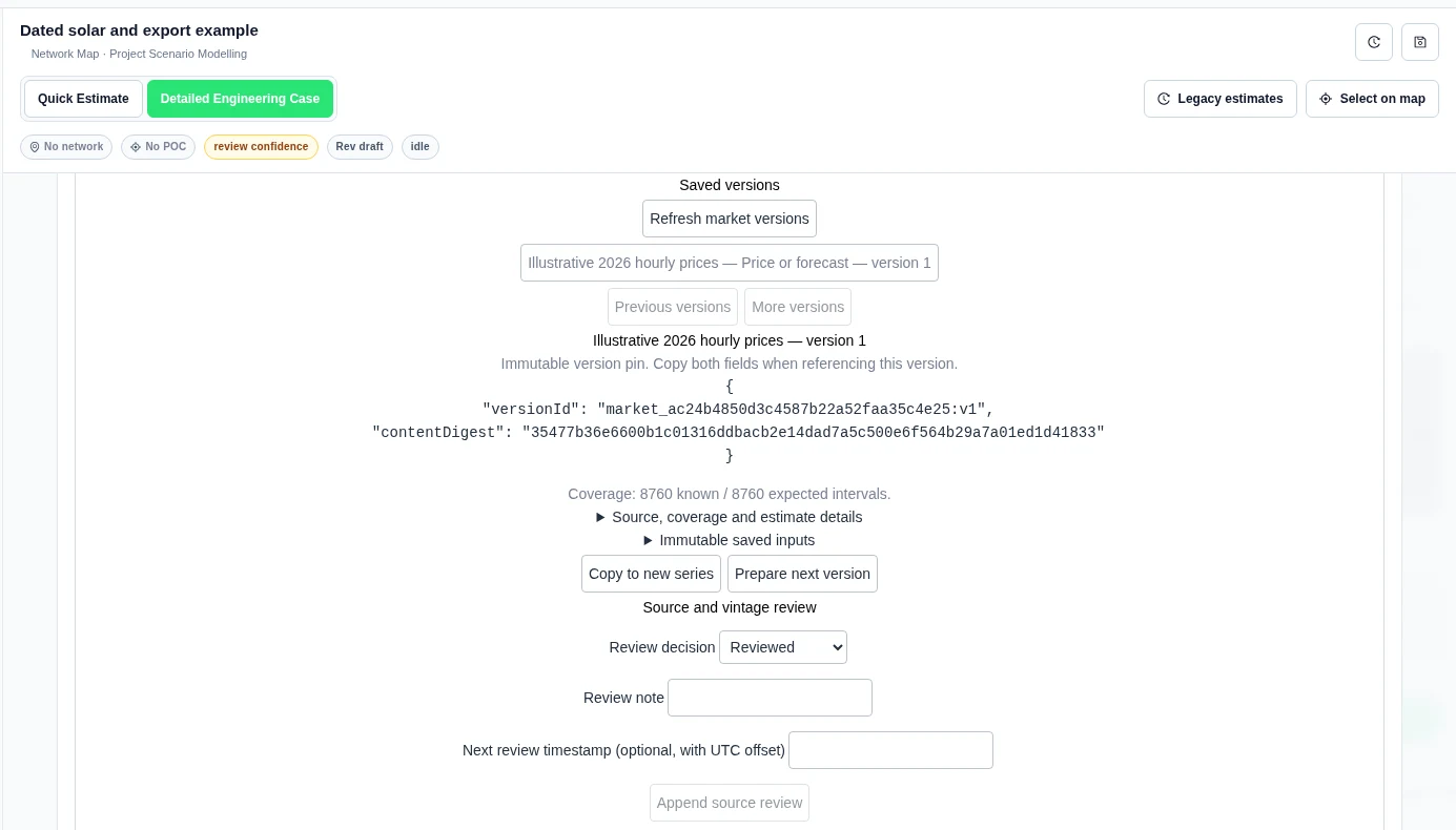
Our example was an explicitly labelled forecast assumption: 50 AUD/MWh for each hourly interval in 2026, in UTC. It was authored for this guide. Standalone market estimates do not change dispatch.
Save and pin commercial terms
- Under Saved commercial instruments, select Open commercial library, then New blank instrument.
- Set Instrument name, Saved contract type, Energy basis and Accounting. Supply the term dates, currency, timezone, volume provenance and contract terms. Use Advanced instrument JSON and schema for structured fields.
- Select an exact Price version where needed. Do not invent a version ID or digest.
- Select Save instrument. Choose its exact Instrument version, then Pin selected version to case.
- Check Case instrument pins. Select Save case revision to retain the pin.
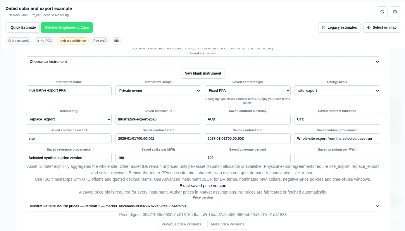
Saved contract types include fixed PPA, behind-the-meter PPA, physical or financial CfD, shaped swap and demand response. Set the behind-the-meter rate as an explicit contract assumption.
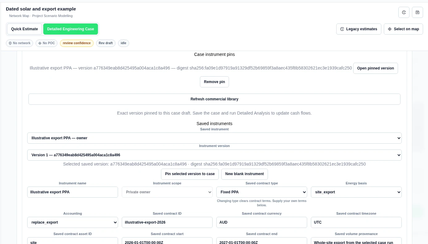
Worked example: an export PPA pin
We saved Illustrative export PPA version 1. It used AUD, UTC, a 2026 term, strike 100 AUD/MWh, coverage 100%, site_export and replace_export. We selected the saved synthetic hourly price version above. The case showed the instrument’s exact version and digest after pinning.
Read saved case settlement
Run a Detailed Engineering Case with reviewed chronological profiles and the saved pins. Under Value → Detailed commercial settlement, check status, currency, model year, amount and reasons. Use Export full commercial settlement JSON for the full evidence. Check the resulting case cash flows before relying on a return metric.
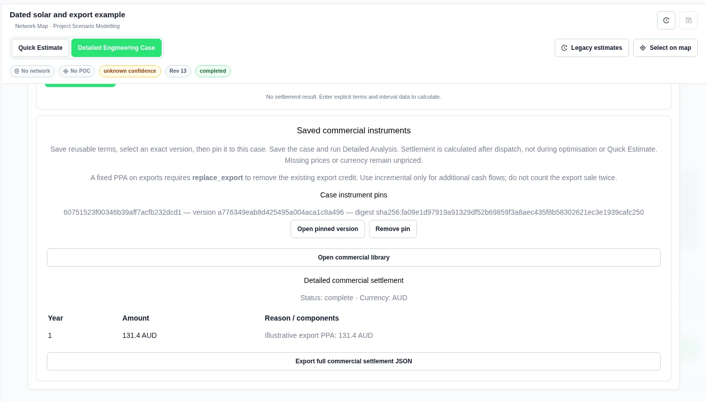
Worked example: positive settlement in case cash flows
We ran the saved Illustrative export PPA pin above in a one-year, hourly 2026 case. The case used AUD and UTC, 1 kW constant load and 2 kW solar. Its synthetic solar resource was 1 pu for hours 10:00–15:00 UTC each day and 0 otherwise. The completed run used provided profiles and exported 2.19 MWh. The scalar export credit was 0.04 AUD/kWh. No exact tariff was pinned.
The saved PPA covered 100% of site export at 100 AUD/MWh with replace_export accounting. Detailed commercial settlement returned complete. Its 8,760-row JSON export supplied these money legs:
| Saved settlement component | Amount (AUD) |
|---|---|
| Fixed energy payment | 219.00 |
| Replaced export credit | −87.60 |
| Net adjustment added to case cash flows | 131.40 |
These totals are sums of the exported interval rows. For the hour starting 2026-01-01T10:00:00+00:00, the product supplied 0.001 MWh, a 0.10 AUD fixed payment and a −0.04 AUD replaced credit. The net adjustment was 0.06 AUD. All rows retained estimate: true. Complete means the requested model calculation completed.
Check the case result, not only the contract amount
Open Results → Economics → Cashflow explorer and choose Annual model years. In this example, 1,000 AUD initial capital cost and 20 AUD first-year operating cost were explicit inputs. The discount rate was 8%. The case returned:
| Case result | Amount (AUD) |
|---|---|
| Year 1 revenue and savings, after settlement | 766.50 |
| Year 1 net cash flow | 746.50 |
| Lifetime net cash flow, including initial investment | −253.50 |
| Lifetime discounted cash flow | −308.80 |
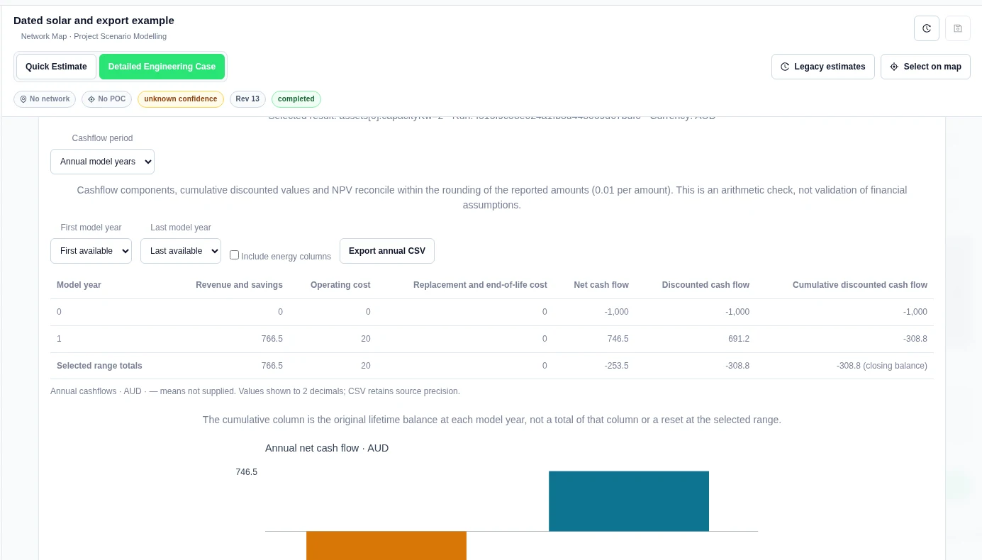
The positive contract adjustment does not make this one-year investment profitable. In Monthly view, the annual contract adjustment appears at year end, not as monthly payments. See Value and Finance for the monthly, quarterly and fiscal-year views.
Calculate a standalone draft instead
The separate Contract settlement · draft only panel values supplied interval observations without saving a commercial instrument. Its result is not added to case economics or dispatch. Draft inputs are discarded when you leave that section. Export the result before leaving if you need it.
Enter terms and observations
- Choose Contract type.
- Enter Contract ID, Contract currency, Contract timezone, Contract start and Contract end. Use explicit ISO timestamps with Z or a UTC offset. The start is inclusive; the end is exclusive.
- Enter Asset ID where required. A Participant ID is an optional tag, not an allocation rule.
- State Volume provenance and, where required, Reference price provenance. Label assumed values as assumptions.
- Enter the price or demand-response terms. Use Interval length (minutes) from 1 to 60.
- Supply observations in Intervals JSON. Use quoted decimal strings for energy and prices.
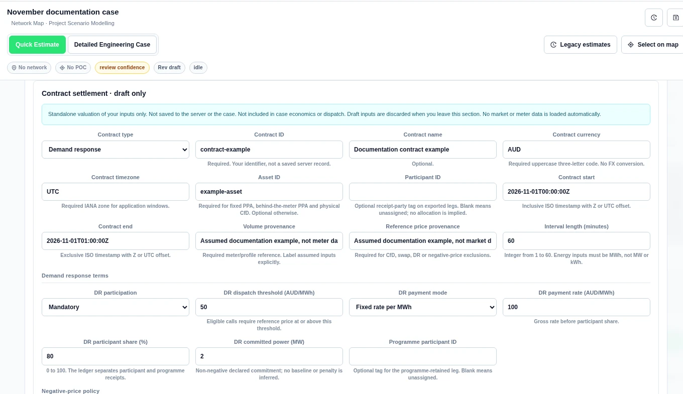
Energy is MWh, not MW or kWh. Prices are in the contract currency per MWh. Use sorted, unique, non-overlapping intervals. The request limit is 17,568 rows. Missing observations stay missing; do not replace them with zero.
Calculate and review the ledger
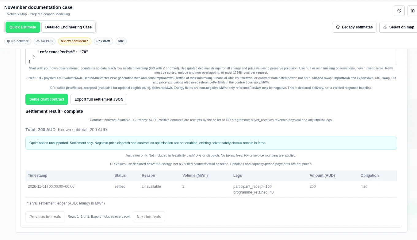
- Select Settle draft contract.
- Read Settlement result, Total, Known subtotal and each interval’s status.
- Review the separate money legs and any missing-data reasons.
- Select Export full settlement JSON before leaving the section if you need the result. The export includes all rows, not just the displayed page.
Worked examples: fixed price and differences
All examples below used Contract currency AUD, Contract timezone UTC and a single 60-minute interval starting 2026-11-01T00:00:00Z. The contract ended at 2026-11-01T01:00:00Z. The observations were labelled documentation assumptions.
For the PPA and CfD examples, we used strike 100 AUD/MWh, premium 0, coverage 100%, Seller receives, no payment floor or cap, and Include all prices. The interval was:
[{"timestamp":"2026-11-01T00:00:00Z","volumeMwh":"2","referencePerMwh":"70"}]| Contract type | Product money legs | Total (AUD) |
|---|---|---|
| Fixed PPA | fixed_energy_payment: 200 | 200 |
| Physical CfD | physical_market_receipt: 140; cfd_adjustment: 60 | 200 |
| Financial CfD | cfd_adjustment: 60 | 60 |
| Shaped swap | cfd_adjustment: 60 | 60 |
For Shaped swap, replace volumeMwh with importMwh "3" and exportMwh "1". Keep the same reference price. The product settled the 2 MWh net volume. A financial CfD records the adjustment, not the physical energy sale. The physical CfD already includes its market leg; do not add that leg again in a portfolio.
Worked example: demand response
Select Demand response. Use the same currency, timezone and hour. Set DR participation to Mandatory, dispatch threshold to 50 AUD/MWh, payment mode to Fixed rate per MWh, payment rate to 100 AUD/MWh, participant share to 80% and committed power to 2 MW. Supply:
[{"timestamp":"2026-11-01T00:00:00Z","called":true,"deliveredMwh":"2","referencePerMwh":"70"}]The product returned participant_receipt 160 AUD and programme_retained 40 AUD. Total and known subtotal were both 200 AUD. The obligation was met. This example uses declared delivery inputs.
Standalone draft limits
- No contract or negative-price dispatch optimisation is performed.
- No taxes, fees, currency conversion or invoice rounding are applied.
- Demand-response penalties and capacity-period payments are not priced.
- Negative-price run policies require a complete regular time axis. Qualifying prices are strictly below the selected threshold.
- Payment collars apply to the payment rate, not the reference price.
- An unavailable result is not zero. Review interval status as well as any known subtotal.
Choose among saved market venues
- In Value → Saved commercial instruments → Open commercial library, choose Market participation estimate.
- Under Market participation and shared capacity, choose venue, a direction and explicit capacity evidence. Select the exact saved Price version. State transfer efficiency.
- Save and pin each venue version. Save the case and run a Detailed Engineering Case.
- Read Detailed commercial settlement. Select Export full commercial settlement JSON to inspect venueChoiceRank and effectivePricePerMwh.
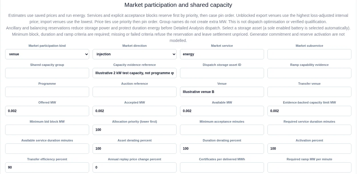
Exports rank by price multiplied by transfer efficiency, highest first. Imports rank by price divided by efficiency, lowest first. Signed and zero prices retain their meaning. Services and explicit acceptance blocks reserve capacity first, by priority then saved pin order. Ties use that same order. A later venue may receive unused capacity. Import and export cohorts are not price-compared or netted against each other.
Worked example: two export venues
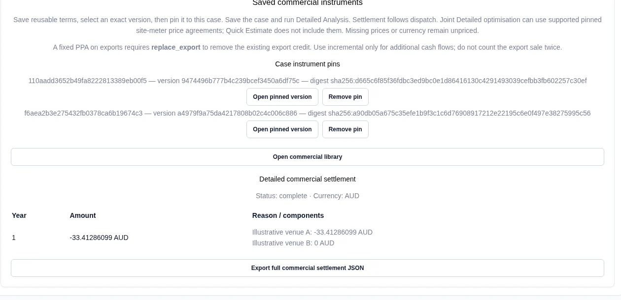
We pinned two example 2026 venues, both priced at 50 AUD/MWh. Each declared 0.002 MW capacity. Venue A used 100% transfer efficiency; B used 90%. The full export ranked A first at 50 AUD/MWh and B second at 45 AUD/MWh. At 12:00 UTC on 1 January, A received 0.002 MW of shared capacity and 0.000052121 MWh of dispatched export. B received 0 MW and 0 MWh.
The completed year's net adjustment was −33.41286099 AUD for A and 0 AUD for B. This is an adjustment, not gross revenue: replace_export removed the case's 0.08 AUD/kWh credit and added the lower venue receipt. All inputs and receipts were estimates.
Reserve storage capacity for ancillary services
- Choose ancillary or balancing under Market participation kind.
- Set Dispatch asset ID. Enter a storage asset, or a supported dispatchable biomass or hydro generator. A sole enabled battery can be selected automatically. Specify direction, accepted capacity, minimum block, service duration, available duration, required and available ramp, and evidence.
- Save and pin the version. Save and rerun the Detailed case.
- In the settlement export, inspect dispatchReservation, its status and reason.
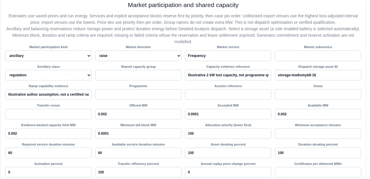
Both directions share one converter power pool. Reserved power reduces charging and discharging limits. Duration SOC is protected at interval start and end. Raise service also reserves daily discharge throughput. The remaining daily budget becomes a conservative uniform discharge-power ceiling; it can restrict peak output more than a dynamic optimiser would.
We explicitly set Accepted MW and Minimum bid block MW to 0.0001 MW (0.1 kW), below the 2 kW / 4 kWh battery maximum. The 60-minute raise reservation was set by that authored accepted block, not clipped to 0.1 kW by power, SOC or throughput. Offered, available and evidence-backed capacity were 0.002 MW. Required and available ramp were both 0.0001 MW per minute. The export returned status: reserved, qualificationCheck: modelled and the named storage asset. The test used an explicit 0% activation assumption and returned 0 AUD ancillary receipt.
Model demand-response events
- Choose Demand response as the saved contract type.
- In Response baseline and capacity, choose Estimate from earlier case intervals. Set History day rule, Lookback days and Minimum sample days.
- Enter committed response, price threshold, payment, participant share, shortfall penalty and optional tolerance from the agreement.
- Select Add response event for each called interval. Use timestamps with UTC offsets. State acceptance where needed. Confirm Event schedule is complete only after listing every event.
- Save and pin the version. Run Detailed mode and inspect responseBaseline and responseCompliance in the full settlement export.
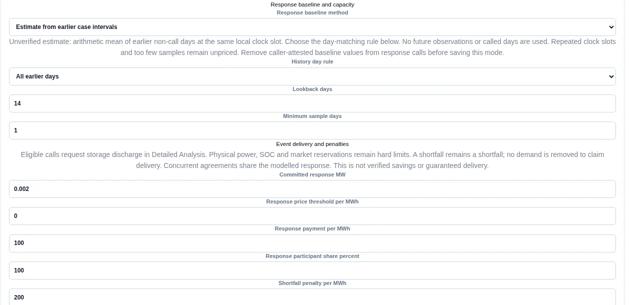
The history rules use the same local clock slot on all earlier eligible days, the same weekday/weekend type, or the same day of week. Called days, missing imports and repeated clock slots are excluded. Too few samples leave the baseline unknown. User-attested baselines also remain unverified unless external verification metadata is supplied. That metadata is still user-supplied, not checked independently by Network Map.
Worked example: a modelled shortfall stays visible
We added a mandatory one-hour event at 18:00 UTC on 5 January 2026. The example terms committed 0.002 MW, paid 100 AUD/MWh and charged 200 AUD/MWh of shortfall. The case-history rule used all earlier days, a 14-day lookback and one required sample day.
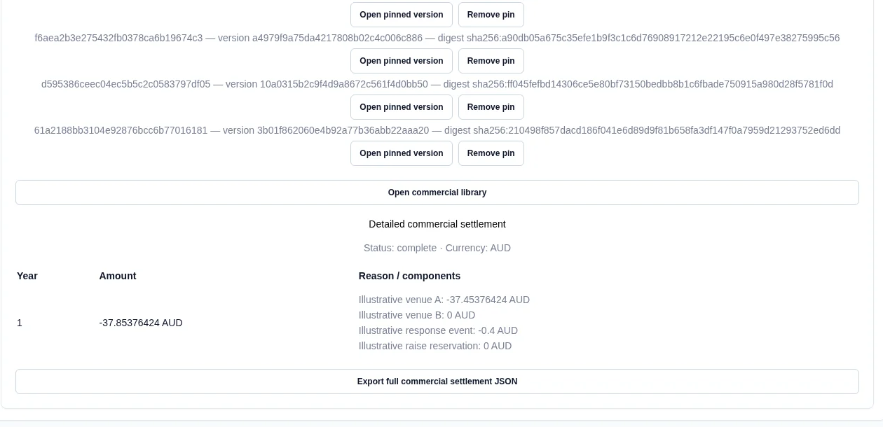
The product found 4 sample days, with an unverified baseline of 0.8708333333333333 kW. Required energy was 0.002 MWh. Delivered response was 0 MWh; shortfall was 0.002 MWh. The penalty was 0.400 AUD and the settlement leg was −0.400 AUD. The combined venue, reserve and response adjustment was −37.85376424 AUD.
Choose the negative-price dispatch rule
- Open a supported saved site-meter agreement and its Negative-price dispatch section.
- Set Negative-price exclusion, consecutive intervals and raw reference threshold.
- Choose Optimiser action: Exclude payment; allow merchant export, or Require zero site export during exclusions.
- Save a new instrument version and pin it. Enable Use joint optimisation in Detailed Analysis in Options. Save and run.
- Read the joint diagnostic. A rule-based fallback does not enforce the joint zero-export constraint.
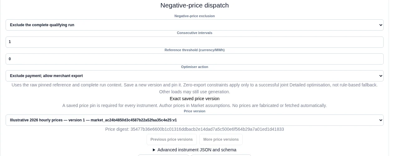
During a zero-export exclusion, generation can still serve load or charge storage. Supported joint terms include linear site-meter fixed PPAs, physical CfDs and financial CfDs. The saved joint diagnostic records which pinned terms were included in the dispatch objective. See Dispatch Calendars and Sizing before relying on the optimiser.
Settle a modelled CfD
- Open Value → Saved commercial instruments → Open commercial library. Choose Modelled CfD as the Saved contract type.
- Enter the contract dates, currency, timezone, strike and coverage. Select CfD volume basis and CfD reference price. For a wholesale reference, choose an exact saved Price version.
- Enter CfD interval (minutes) and the payment floor and cap. Choose Payment direction, then Save instrument.
- With a completed saved Detailed run selected, choose Settle modelled CfD against saved run.
- Open Modelled rules and interval results. Use Export modelled results JSON to keep the evidence.
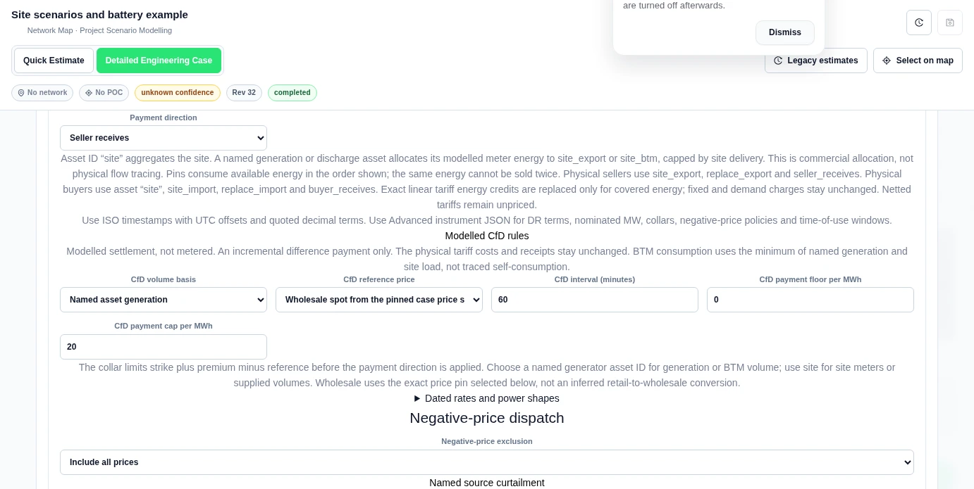
The calculation uses strike plus premium minus reference. The payment collar applies before payment direction. Volume and coverage then scale the payment. Named generation, behind-the-meter consumption, site import, site export and supplied volumes are explicit choices.
Worked example: a capped difference payment
We selected Named asset generation for solar, a pinned example wholesale reference of 50 AUD/MWh, a strike of 80 AUD/MWh, 100% coverage and Seller receives. The payment floor was 0 AUD/MWh and the cap was 20 AUD/MWh. The case used 60-minute intervals from 1 January 2026 to 1 January 2027.
The completed saved-run calculation returned 64.822302660 AUD. This is the modelled incremental difference payment. The saved run retains its physical energy flows and tariff accounting.
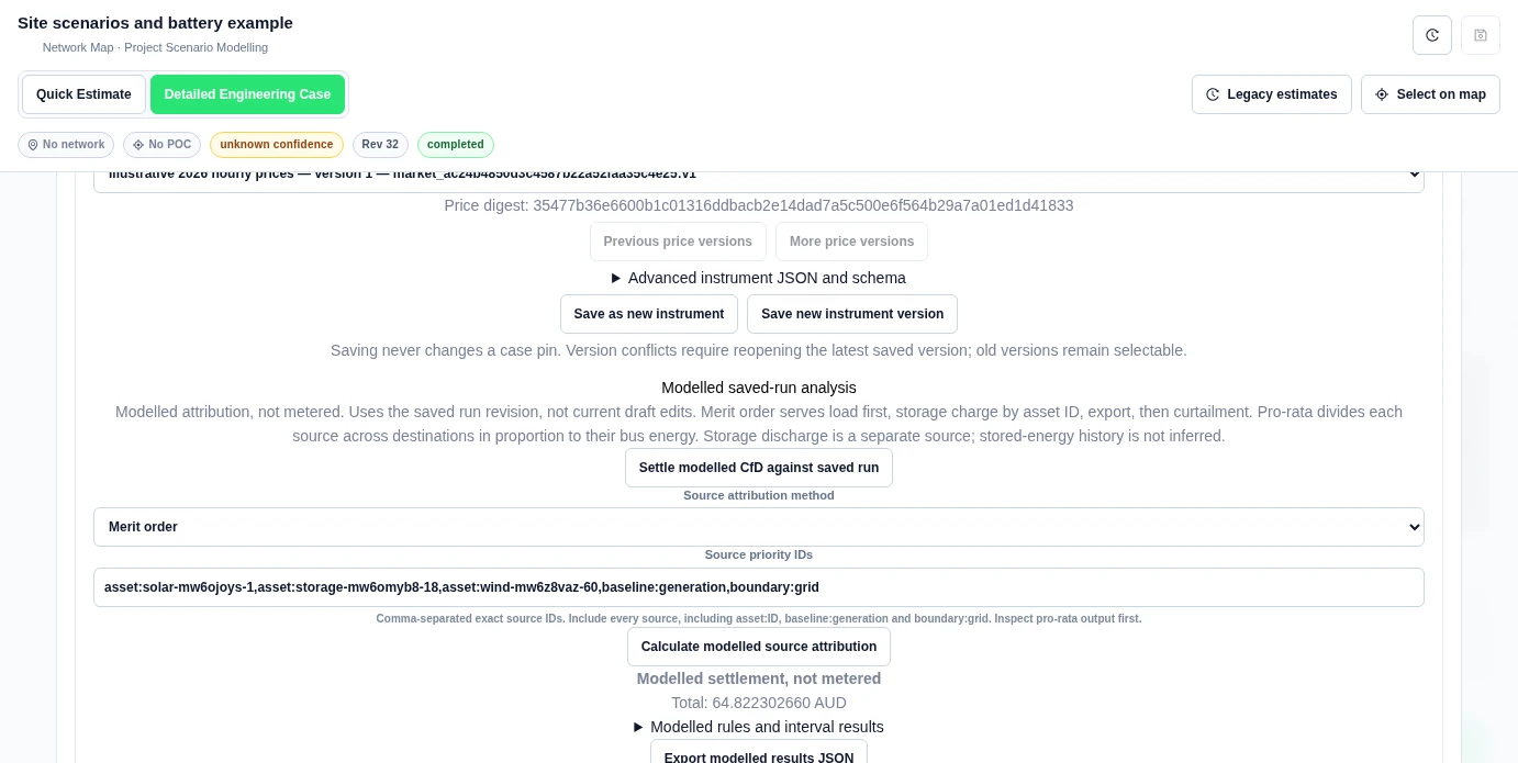
Review modelled source attribution
- Keep the saved Detailed run selected. In Value → Modelled saved-run analysis, choose Source attribution method → Pro-rata.
- Select Calculate modelled source attribution. Open Modelled rules and interval results to inspect the exact source IDs.
- For Merit order, enter all source IDs in Source priority IDs, in your preferred order. Calculate again.
- Export the result JSON to keep every interval and source-to-destination path.
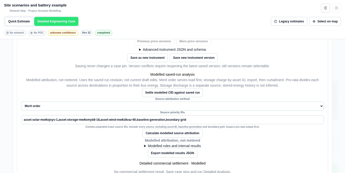
Worked example: two allocation methods
At 00:00 UTC on 1 January 2026, pro-rata attributed 0.6443468797493633 kWh of solar and 0.3556531202506367 kWh of wind to served load. With solar first in merit order, solar supplied 1 kWh to served load and 0.23414942676713513 kWh to the battery. Wind supplied 0.6812 kWh to the battery. Both reports cover 8,760 intervals from the same saved run.
Set a modelled named-source curtailment rule
- Open your Saved instrument. Set its Negative-price exclusion and exact Price version.
- Under Named source curtailment, choose Require zero source generation during exclusions. Enter the Curtailable generation asset ID and select the Source exclusion scope.
- Save the instrument version and pin it to the case. In Options, enable Use joint optimisation in Detailed Analysis. Save and run the Detailed case.
- Read the saved commercial settlement and the joint-dispatch-objective in the JSON manifest.
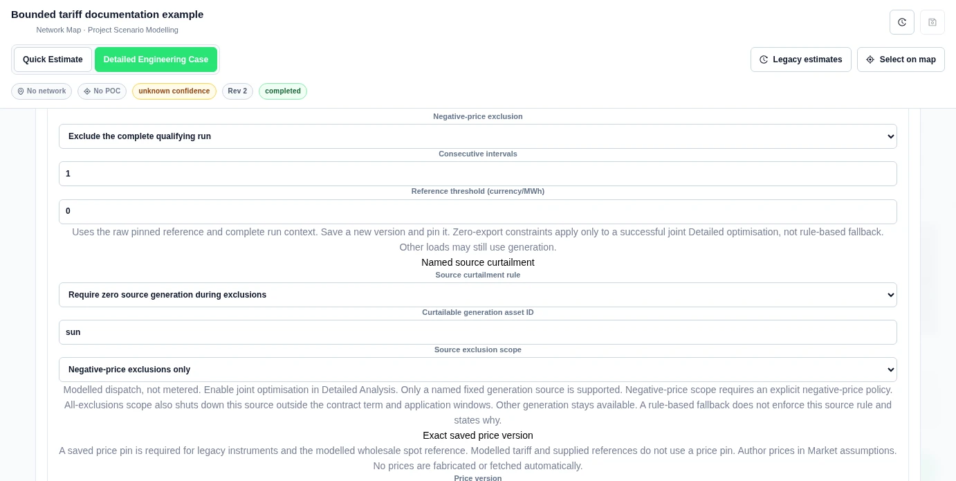
Worked example: curtail one of two solar sources
We supplied two example 3 kW solar sources across four one-hour UTC intervals. A modelled CfD used the named source sun, a 300 AUD/MWh strike, and pinned reference prices of −10, 50, 50 and 50 AUD/MWh. The policy excluded the complete qualifying run below 0 AUD/MWh.
The saved joint result returned optimal. Named-source curtailment was 3, 0, 0 and 0 kWh. The other source remained available. Commercial settlement was 2.25 AUD, with a 0 AUD difference between the solver and exact settlement.
Modelled dispatch. This source rule is applied by joint optimisation. Use the saved optimiser status and source ledger to review the result.
Trade across time and venues with joint dispatch
- Save each price series in Market assumptions.
- In Saved commercial instruments, select Market participation estimate and Market participation kind → venue. Use Market direction → withdrawal for imports or injection for exports. Enter Accepted MW and Available MW.
- Pin each instrument version to the case. Enable Use joint optimisation in Detailed Analysis in Options, then save and run.
- Review marketTrading and the joint objective in the saved JSON manifest. Use Export full commercial settlement JSON for interval settlement.
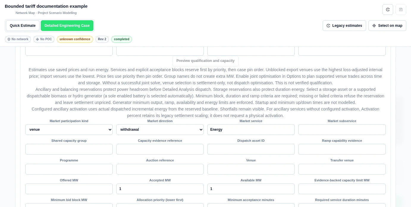
Worked example: three venues and one battery
The example battery had 1,000 kW power, 2,000 kWh capacity, 100% charge and discharge efficiency, and zero opening and terminal SOC. Load was zero across four one-hour UTC intervals on 1 January 2026. Import and export limits were each 1,000 kW.
| Price source, AUD/MWh | Hour 1 | Hour 2 | Hour 3 | Hour 4 |
|---|---|---|---|---|
| Import venue | 20 | 20 | 200 | 200 |
| Export venue A | 10 | 10 | 160 | 10 |
| Export venue B | 10 | 10 | 10 | 170 |
The saved result was optimal. Grid imports were 1,000, 1,000, 0 and 0 kW. Exports were 0, 0, 1,000 and 1,000 kW. Export venue A received the third-hour volume and B received the fourth-hour volume.
The joint objective was −290 AUD. The commercial adjustment was 890 AUD against the case's 0.3 AUD/kWh import assumption and 0 AUD/kWh export assumption. The adjustment is a replacement-accounting leg, not a second trading receipt.
Model ancillary activation
- In Market participation and shared capacity, select ancillary. Supply the capacity, block, duration, ramp evidence and Dispatch asset ID.
- Under Ancillary activation, enter Activation probability percent or a dated Activation profile JSON. Enter Activation price per MWh and pin a capacity-price source.
- Save and pin the instrument version. Run the Detailed Engineering Case. Inspect requested, delivered and shortfall energy in Export full commercial settlement JSON.
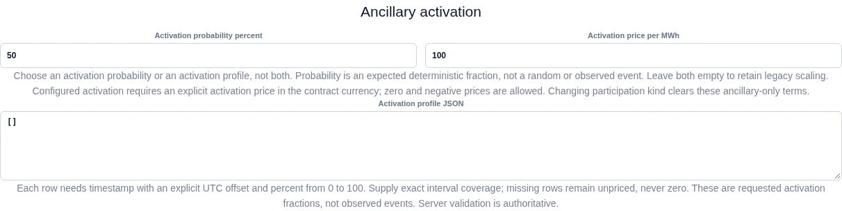
Worked example: expected raise activation
We supplied two hourly intervals with 20 kW load. One 10 kW / 40 kWh battery started at 50% SOC. The example reserve was 0.004 MW, with a 0.001 MW minimum block, 60-minute duration, a required ramp of 0.001 MW/min and available ramp of 0.002 MW/min. Capacity price was 50 AUD/MW/h.
At 50% expected activation and 100 AUD/MWh, each interval delivered 0.002 MWh, with 0 MWh shortfall. Discharge increased from the computed 6 kW baseline to 8 kW. Each interval settled 0.400000000000 AUD. The two-interval total was 0.8 AUD.
This is a modelled expected fraction. The example uses one active storage asset and supplied operating limits.
Model balancing up and down
- Select Market participation kind → balancing. Set Market direction, Balancing action, Dispatch asset ID and Activation percent.
- Supply the capacity, minimum block, duration, ramp evidence and exact price version. Save and pin the instrument version.
- Run the Detailed case. Read the computed baseline, executed action and delivered energy in Export full commercial settlement JSON.
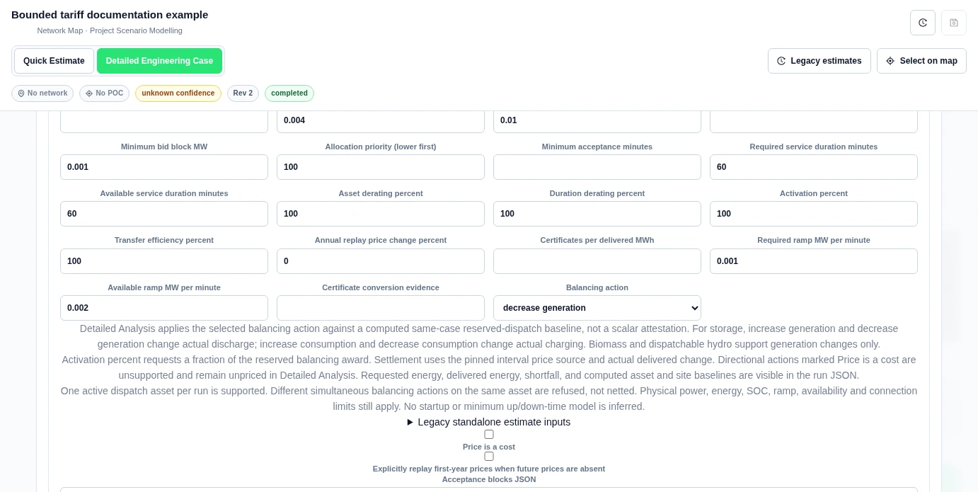
Worked example: separate increase and decrease runs
We used the same two-hour load and 10 kW / 40 kWh battery. Each separate run had a 0.004 MW award, 100% activation and an example 50 AUD/MWh price.
| Action | Baseline discharge | Executed discharge | Delivered per interval | Settlement per interval |
|---|---|---|---|---|
| increase_generation | 6 kW | 10 kW | 0.004 MWh | 0.200000000000 AUD |
| decrease_generation | 6 kW | 2 kW | 0.004 MWh | 0.200000000000 AUD |
Both runs returned 0 MWh shortfall in each interval. Each two-hour settlement total was 0.4 AUD. The baseline came from the same case's reserved dispatch. These are modelled storage actions.
Import Nordic day-ahead snapshots
Open Design, find Scheme sources and connection access, then select Open Nordic snapshot importer. Choose the Price dataset, Country and bidding zone, Price currency and Source format.
Enter the snapshot start, end and retrieval timestamps with UTC offsets, plus the Official snapshot request URL. Upload the Official snapshot file or paste its content. Select Preview native day-ahead prices.
This worked example uses an actual Energinet DayAheadPrices snapshot for Denmark DK1. The selected window is 7 November 2025 at 23:00 UTC to 8 November 2025 at 01:00 UTC. The preview contains 8 of 8 quarter-hour prices in EUR/MWh. The first interval is 102.320000 EUR/MWh; the last is 93.339996 EUR/MWh.
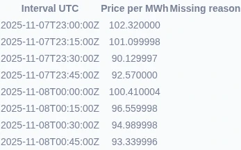
Use Download attributed prices CSV or Download price library inputs to retain the price data and source record. Expand Source manifest to review the selected window, currency, interval length, source digest and licence.
Compare declared capacity quantities
In Value, select Open commercial library and open a market participation instrument. Find Capacity accreditation and source edition. Supply Nominal power MW, Accredited power MW and Accreditation evidence. Enter the offered, accepted and available capacity in the market participation fields.
Set Accepted capacity basis to match the supplied award. For an already accredited award, use 100% for both asset and duration derating. Enter the Qualification interval start with UTC offset and Qualification interval minutes, then select Preview qualification and capacity.
This modelled preview has 0.01 MW nominal, 0.008 MW caller-accredited, 0.006 MW offered and 0.004 MW awarded. Physical availability is 0.01 MW. The preview requests and allocates 0.004 MW for the supplied one-hour interval. The supplied award is already accredited, so it receives no second derating.