

Docs Menu
Worked Examples
Build saved cases for solar, storage, and network-tariff screening. These examples use synthetic assumptions and show the model outputs returned for those inputs.
For a size sweep with a different load and cost basis, jump to Riverbend cold store: nine solar and battery designs.
Before you start
Open Project Modelling. Follow Scope, Profiles, Design, Value, Options, Run, and Results. Use Save case revision to save each case. Use Case history to reopen it. Save your current work before starting another case.
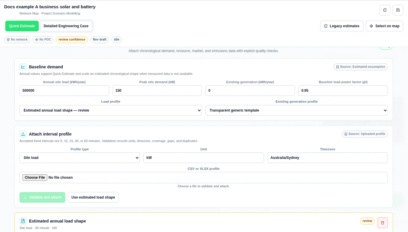
Examples A–D use the inputs below as well as their own inputs table. The demand profile is generated with Use estimated load shape. No CSV upload is needed. The profile card marks the estimate for review.
Shared inputs
| Input | Value |
|---|---|
| Currency | AUD |
| Annual site load | 500000 kWh/year |
| Peak site demand | 150 kW |
| Existing generation | 0 kWh/year |
| Baseline load power factor | 0.95 |
| Load profile | Use estimated load shape; synthetic, 30-minute; Australia/Sydney; kW |
| Existing generation profile | Transparent generic template |
| Network input source | Current map; no electrical network or point of connection selected; no snapshot captured |
| Connection direction | Import and export |
| Nominal voltage | 0.4 kV |
| Import limit | 300 kW |
| Export limit | 100 kW (D sweeps 0 and 100 kW) |
| Network screening criteria | Minimum voltage 0.95 pu; maximum voltage 1.05 pu; maximum thermal loading 100%; minimum connection headroom 0 kW; reverse power flow Allowed |
| Analysis horizon | 20 years |
| WACC / discount rate | 8% |
| Inflation | 2.5% |
| Energy escalation / Export escalation | 2% / 2% |
| Opex escalation | 2.5% |
| Quick self-consumption assumption | 70% |
| Export energy value | 0.08 AUD/kWh; example assumption, not supplied by the network tariff |
| FCAS / capacity revenue | 0 AUD/year |
| Grid services capacity revenue | 0 AUD/kW/year |
| Generation capacity value | 0 AUD/kW/year |
| Emissions factor / Carbon value | 0.65 kg CO₂-e/kWh / 0 AUD/t CO₂-e |
| Case decommissioning cost | 0 AUD |
| Chronological value profiles | Flat import value, flat export value, flat emissions factor; none uploaded |
| Ranking metric | NPV |
A. Business solar and battery with a network tariff
This case demonstrates a library tariff and its limits. It is a network-charge-only screening case, not a complete retail bill.
Inputs
| Input | Value |
|---|---|
| Case name | Docs example A business solar and battery |
| Engineering notes | Synthetic business example with annual assumptions and an estimated load shape. |
| Mode | Quick Estimate |
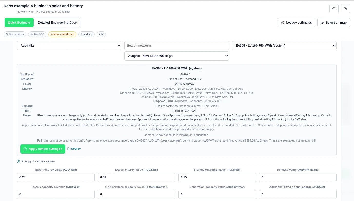
| Network tariff | Australia → Ausgrid → EA305 · LV 160-750 MWh (system), 2026-27; selected manually |
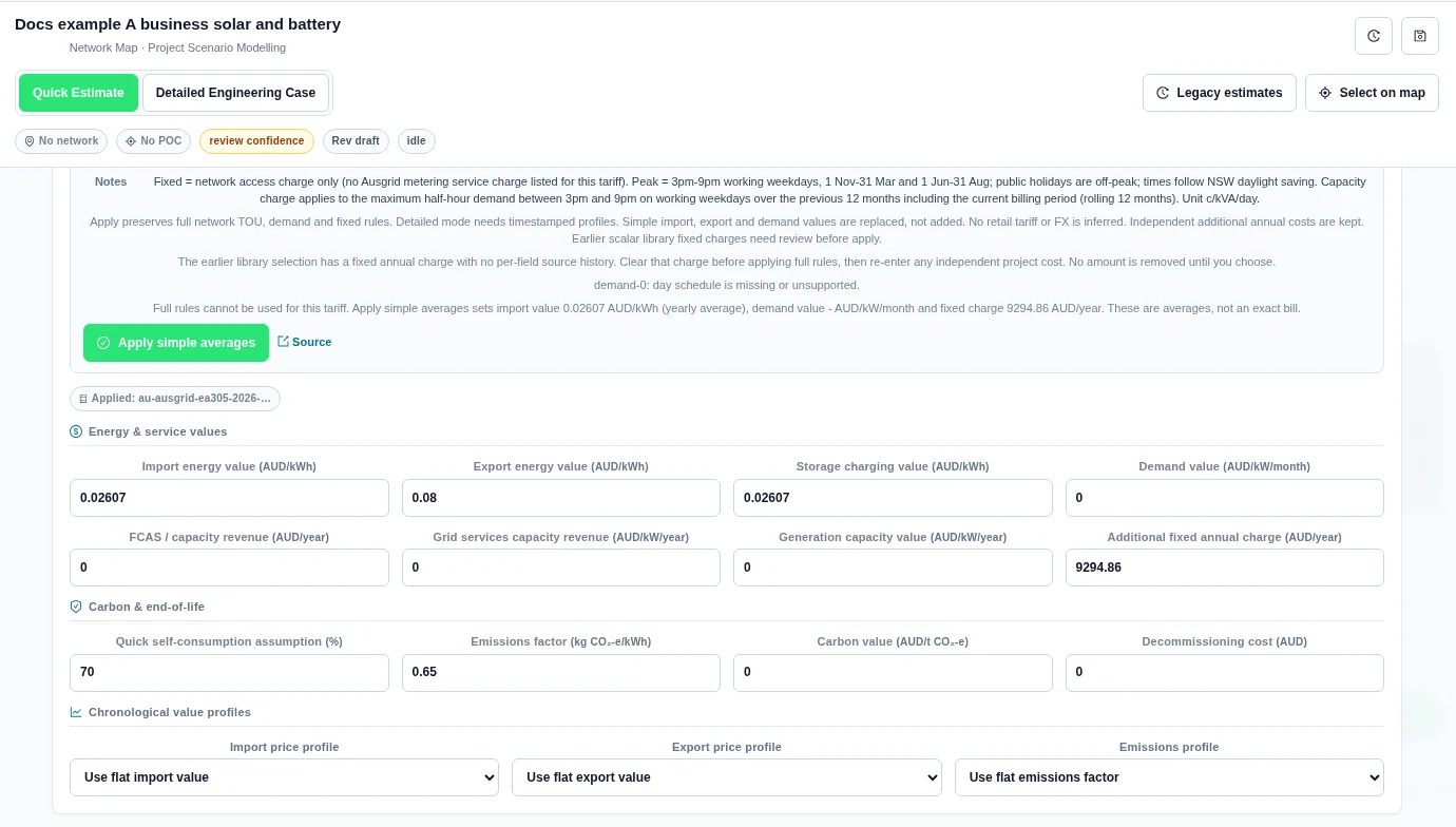
| Tariff application | Apply simple averages; full rules unavailable |
| Import energy value | 0.02607 AUD/kWh; network charges only |
| Storage charging value | 0.02607 AUD/kWh |
| Demand value | 0 AUD/kW/month; library demand rate unavailable |
| Additional fixed annual charge | 9294.86 AUD/year |
| Control policy | Maximise self-consumption |
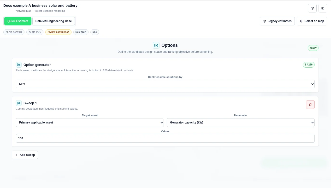
| Sweep 1 | Primary applicable asset; Generator capacity (kW); Values 100 |
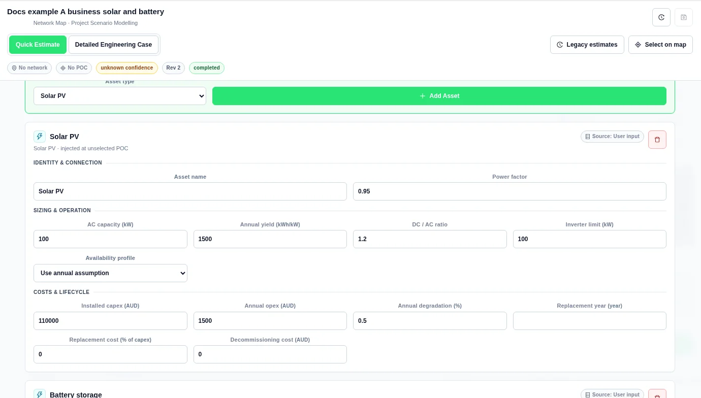
| Solar asset name / Power factor | Solar PV / 0.95 |
| AC capacity / Inverter limit | 100 kW / 100 kW |
| Annual yield / DC / AC ratio | 1500 kWh/kW / 1.2 |
| Availability profile | Use annual assumption; no measured solar profile |
| Solar installed capex / Annual opex | 110000 AUD / 1500 AUD/year |
| Solar annual degradation | 0.5% |
| Solar replacement / Decommissioning | Replacement year blank; replacement cost 0%; decommissioning cost 0 AUD |
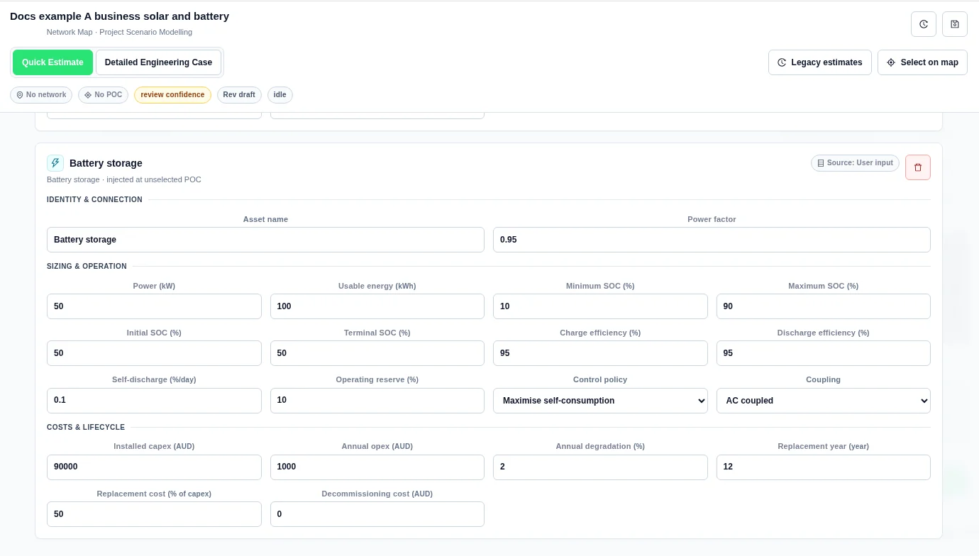
| Battery asset name / Power factor | Battery storage / 0.95 |
| Battery power / Usable energy | 50 kW / 100 kWh |
| Minimum / Maximum SOC | 10% / 90% |
| Initial / Terminal SOC | 50% / 50% |
| Charge / Discharge efficiency | 95% / 95% |
| Self-discharge / Operating reserve | 0.1%/day / 10% |
| Coupling | AC coupled |
| Battery installed capex / Annual opex | 90000 AUD / 1000 AUD/year |
| Battery annual degradation | 2% |
| Battery replacement | Year 12; 50% of battery capex |
| Battery decommissioning cost | 0 AUD |
Steps
- In Scope, name the case and enter the shared connection limits. Keep Quick Estimate selected.
- In Profiles, enter the shared demand values. Set Timezone to Australia/Sydney, then select Use estimated load shape.
- In Design, configure Solar PV. Choose Battery storage and select Add Asset. Enter the sizes and costs above.
- In Value, choose Australia, Ausgrid, and EA305 · LV 160-750 MWh (system).
- Read the tariff card. For this capture it reports demand-0: day schedule is missing or unsupported. Full rules cannot be used. Select Apply simple averages, then set Storage charging value to 0.02607. Leave the separate example export value at 0.08.
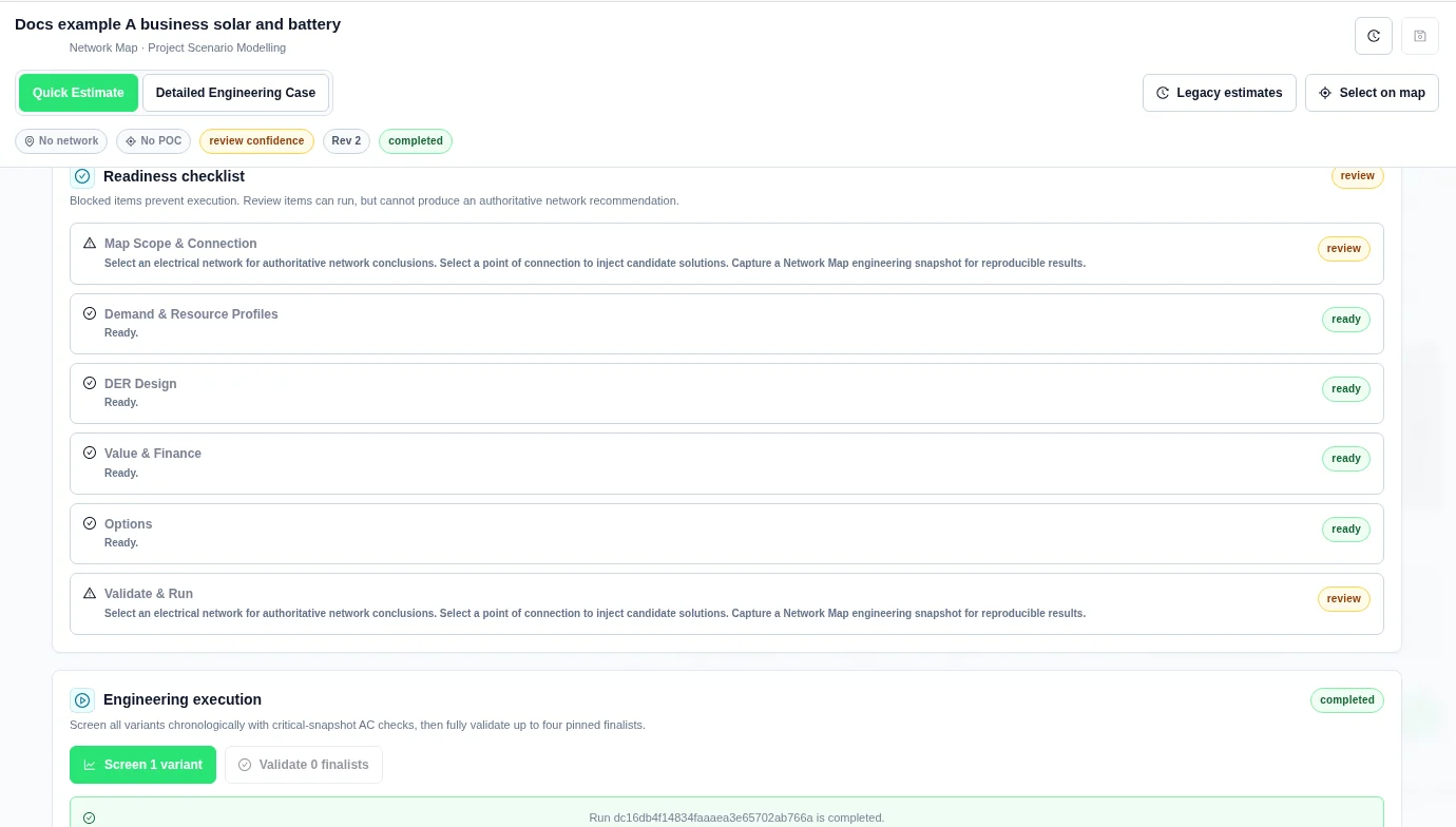
- In Options, set the generator-capacity sweep to 100. Save the case, open Run, and select Screen 1 variant.
- When the run shows completed, open Results, then Summary and Economics.
Results as shown
| Input | Value |
|---|---|
| NPV | -A$300,007 |
| Total capex | A$200,000 |
| First year revenue and savings | A$5,058 |
| First year opex | A$11,795 |
| Annual generation | 150,000 kWh |
| Annual onsite use | 125,440 kWh |
| IRR / Payback | — / — |
| Engineering gate | review |
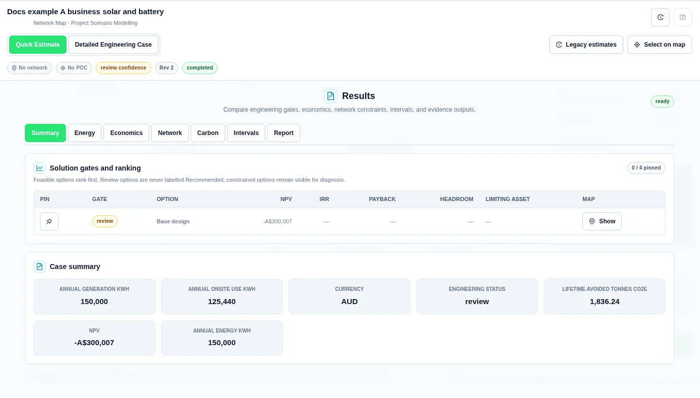
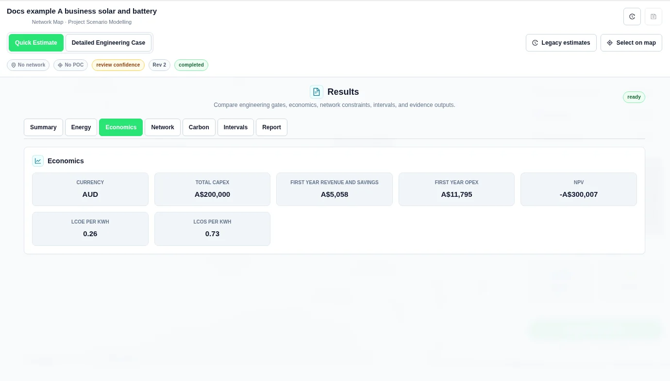
The savings are small because the import value covers network charges only. It does not include the retail energy price. The library is not a complete electricity bill, and its unavailable demand rate contributes no demand value in this case.
The opex inputs are 1500 AUD/year for solar, 1000 AUD/year for the battery, and 9294.86 AUD/year from the tariff's fixed charge. Together they are 11794.86 AUD/year; the product displays A$11,795. This exceeds the displayed first-year savings. Do not treat the negative NPV as a conclusion about the same equipment under a complete retail contract.
B. Solar PV with simple import and export values
This case uses a stated retail import assumption instead of the network-only value in A. It has no battery and no library tariff.
Inputs
| Input | Value |
|---|---|
| Case name | Docs example B solar only |
| Engineering notes | Synthetic business example; simple retail import and export assumptions; no network assessment. |
| Mode | Quick Estimate |
| Network tariff | None selected |
| Import energy value | 0.25 AUD/kWh; example retail import assumption |
| Storage charging value | 0.15 AUD/kWh; unused because no battery |
| Demand value / Additional fixed annual charge | 0 AUD/kW/month / 0 AUD/year |
| Battery | None |
| Sweep 1 | Primary applicable asset; Generator capacity (kW); Values 100 |
| Solar asset name / Power factor | Solar PV / 0.95 |
| AC capacity / Inverter limit | 100 kW / 100 kW |
| Annual yield / DC / AC ratio | 1500 kWh/kW / 1.2 |
| Availability profile | Use annual assumption; no measured solar profile |
| Solar installed capex / Annual opex | 110000 AUD / 1500 AUD/year |
| Solar annual degradation | 0.5% |
| Solar replacement / Decommissioning | Replacement year blank; replacement cost 0%; decommissioning cost 0 AUD |
Steps
- Create the named case in Quick Estimate. Enter the shared scope and profile inputs.
- Keep one Solar PV asset and enter the solar inputs above.
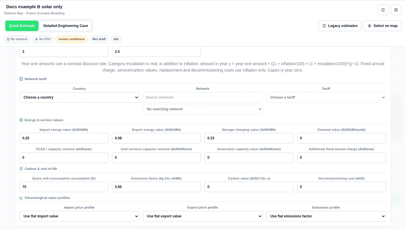
- In Value, leave the network tariff unselected. Set Import energy value to 0.25 and Export energy value to 0.08.
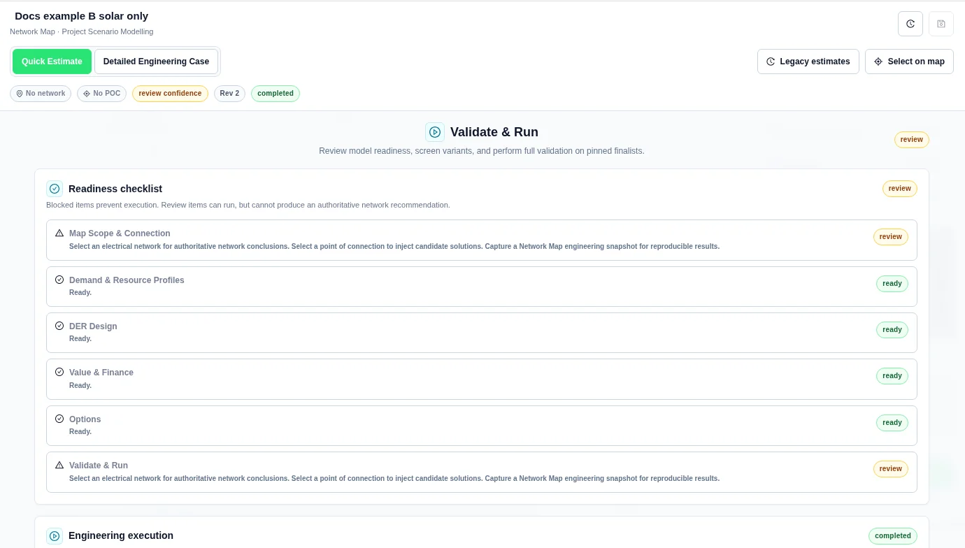
- In Options, use one generator-capacity value: 100. Save the case and select Screen 1 variant in Run.
- Open Results after the run completes.
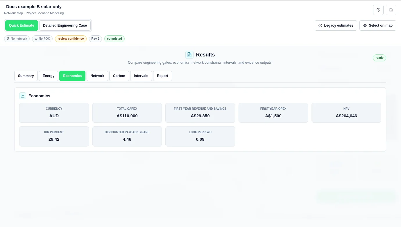
Results as shown
| Input | Value |
|---|---|
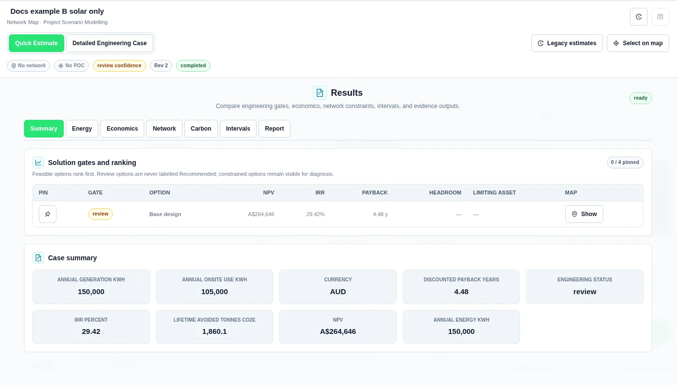
| NPV | A$264,646 |
| IRR | 29.42% |
| Discounted payback | 4.48 y |
| Total capex | A$110,000 |
| First year revenue and savings | A$29,850 |
| First year opex | A$1,500 |
| Annual generation | 150,000 kWh |
| Annual onsite use | 105,000 kWh |
| Engineering gate | review |
Do not compare A and B as a battery investment decision: their import values and fixed charges differ. Keep the same valuation basis when comparing equipment.
C. Battery-only demand-charge screening
This modelled case compares a battery using an annual demand-charge assumption.
Inputs
| Input | Value |
|---|---|
| Case name | Docs example C battery demand reduction |
| Engineering notes | Synthetic business example; peak shaving objective; simple demand charge assumption; no network assessment. |
| Mode | Quick Estimate |
| Network tariff | None selected |
| Solar PV | Removed; no generation asset |
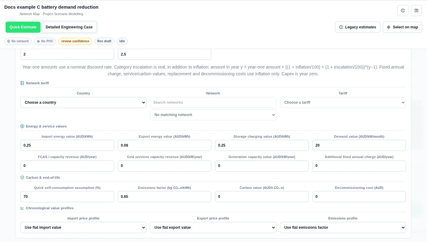
| Import energy value / Storage charging value | 0.25 AUD/kWh / 0.25 AUD/kWh; example retail assumptions |
| Demand value | 20 AUD/kW/month; example assumption |
| Additional fixed annual charge | 0 AUD/year |
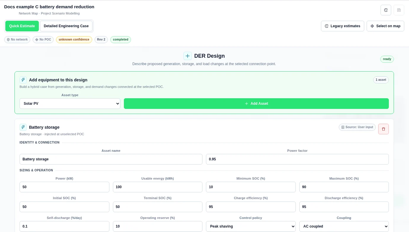
| Control policy | Peak shaving |
| Sweep 1 | Primary applicable asset; Storage power (kW); Values 50 |
| Battery asset name / Power factor | Battery storage / 0.95 |
| Battery power / Usable energy | 50 kW / 100 kWh |
| Minimum / Maximum SOC | 10% / 90% |
| Initial / Terminal SOC | 50% / 50% |
| Charge / Discharge efficiency | 95% / 95% |
| Self-discharge / Operating reserve | 0.1%/day / 10% |
| Coupling | AC coupled |
| Battery installed capex / Annual opex | 90000 AUD / 1000 AUD/year |
| Battery annual degradation | 2% |
| Battery replacement | Year 12; 50% of battery capex |
| Battery decommissioning cost | 0 AUD |
Steps
- Create the named case in Quick Estimate and enter the shared inputs.
- In Design, remove the starting Solar PV asset. Add Battery storage, enter the battery inputs, and set Control policy to Peak shaving.
- In Value, set import and charging values to 0.25 and Demand value to 20. Do not select a library tariff.
- In Options, select Storage power (kW) and enter 50.
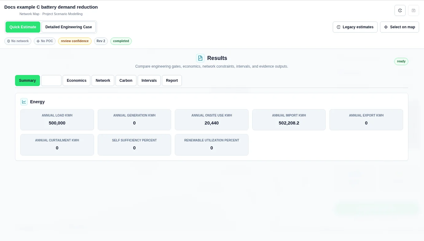
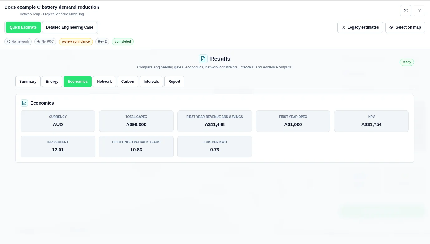
- Save the case. Select Screen 1 variant, then review Summary, Energy, and Economics.
Results as shown
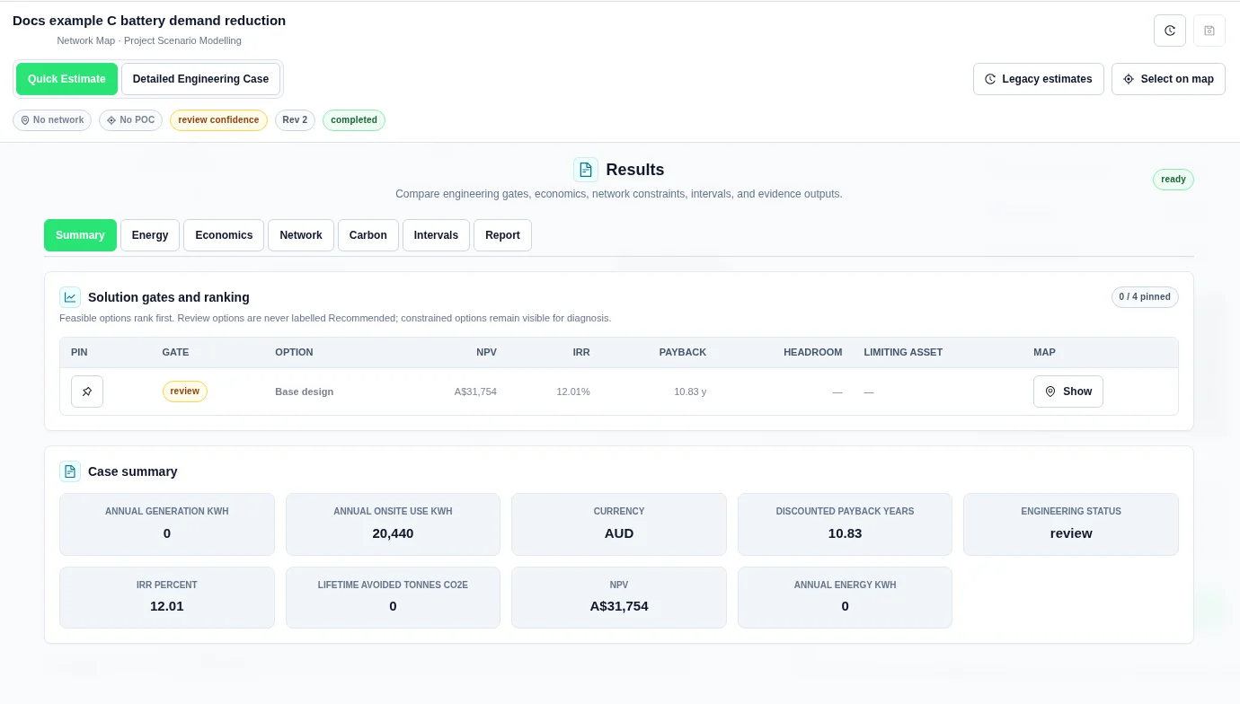
| Input | Value |
|---|---|
| NPV | A$31,754 |
| IRR | 12.01% |
| Discounted payback | 10.83 y |
| Total capex | A$90,000 |
| First year revenue and savings | A$11,448 |
| First year opex | A$1,000 |
| Annual generation | 0 kWh |
| Annual onsite use | 20,440 kWh |
| Annual import | 502,208.2 kWh |
| Annual export | 0 kWh |
| Engineering gate | review |
D. Compare two export-limit options
This comparison keeps equipment and costs fixed and changes the export limit from 0 kW to 100 kW. It uses a stated retail import assumption, not the network-only value in A. Both options include solar and storage.
Inputs
| Input | Value |
|---|---|
| Case name | Docs example D export limit comparison |
| Engineering notes | Synthetic business example; compare export limits 0 and 100 kW for identical equipment and example retail values. |
| Mode | Detailed Engineering Case |
| Network tariff | None selected |
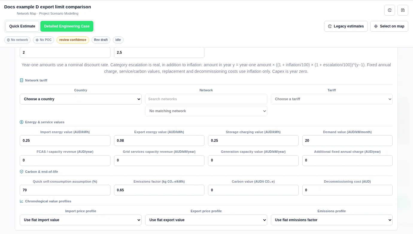
| Import energy value / Storage charging value | 0.25 AUD/kWh / 0.25 AUD/kWh; example retail assumptions |
| Demand value | 20 AUD/kW/month; example assumption |
| Additional fixed annual charge | 0 AUD/year |
| Control policy | Maximise self-consumption |
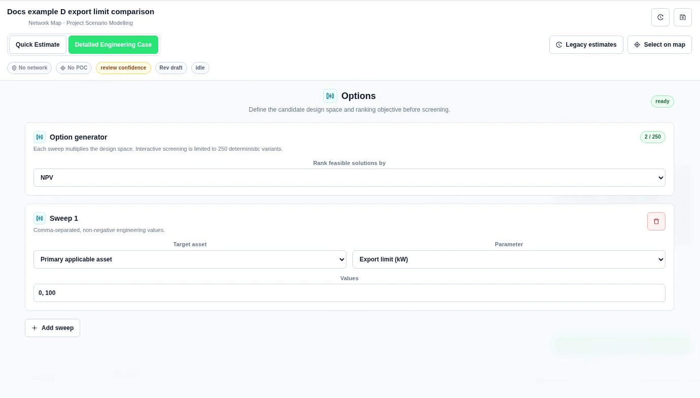
| Sweep 1 | Primary applicable asset; Export limit (kW); Values 0, 100 |
| Solar asset name / Power factor | Solar PV / 0.95 |
| AC capacity / Inverter limit | 100 kW / 100 kW |
| Annual yield / DC / AC ratio | 1500 kWh/kW / 1.2 |
| Availability profile | Use annual assumption; no measured solar profile |
| Solar installed capex / Annual opex | 110000 AUD / 1500 AUD/year |
| Solar annual degradation | 0.5% |
| Solar replacement / Decommissioning | Replacement year blank; replacement cost 0%; decommissioning cost 0 AUD |
| Battery asset name / Power factor | Battery storage / 0.95 |
| Battery power / Usable energy | 50 kW / 100 kWh |
| Minimum / Maximum SOC | 10% / 90% |
| Initial / Terminal SOC | 50% / 50% |
| Charge / Discharge efficiency | 95% / 95% |
| Self-discharge / Operating reserve | 0.1%/day / 10% |
| Coupling | AC coupled |
| Battery installed capex / Annual opex | 90000 AUD / 1000 AUD/year |
| Battery annual degradation | 2% |
| Battery replacement | Year 12; 50% of battery capex |
| Battery decommissioning cost | 0 AUD |
Steps
- Create the named case and select Detailed Engineering Case.
- Enter the shared inputs and the solar and battery inputs above. Keep Maximise self-consumption as the battery policy.
- In Value, set import and charging values to 0.25, export to 0.08, and demand value to 20. These are example retail assumptions; no library tariff is selected.
- In Options, choose Export limit (kW). Enter 0, 100. The equipment and its capex are the same for both options.
- Save the case and select Screen 2 variants.
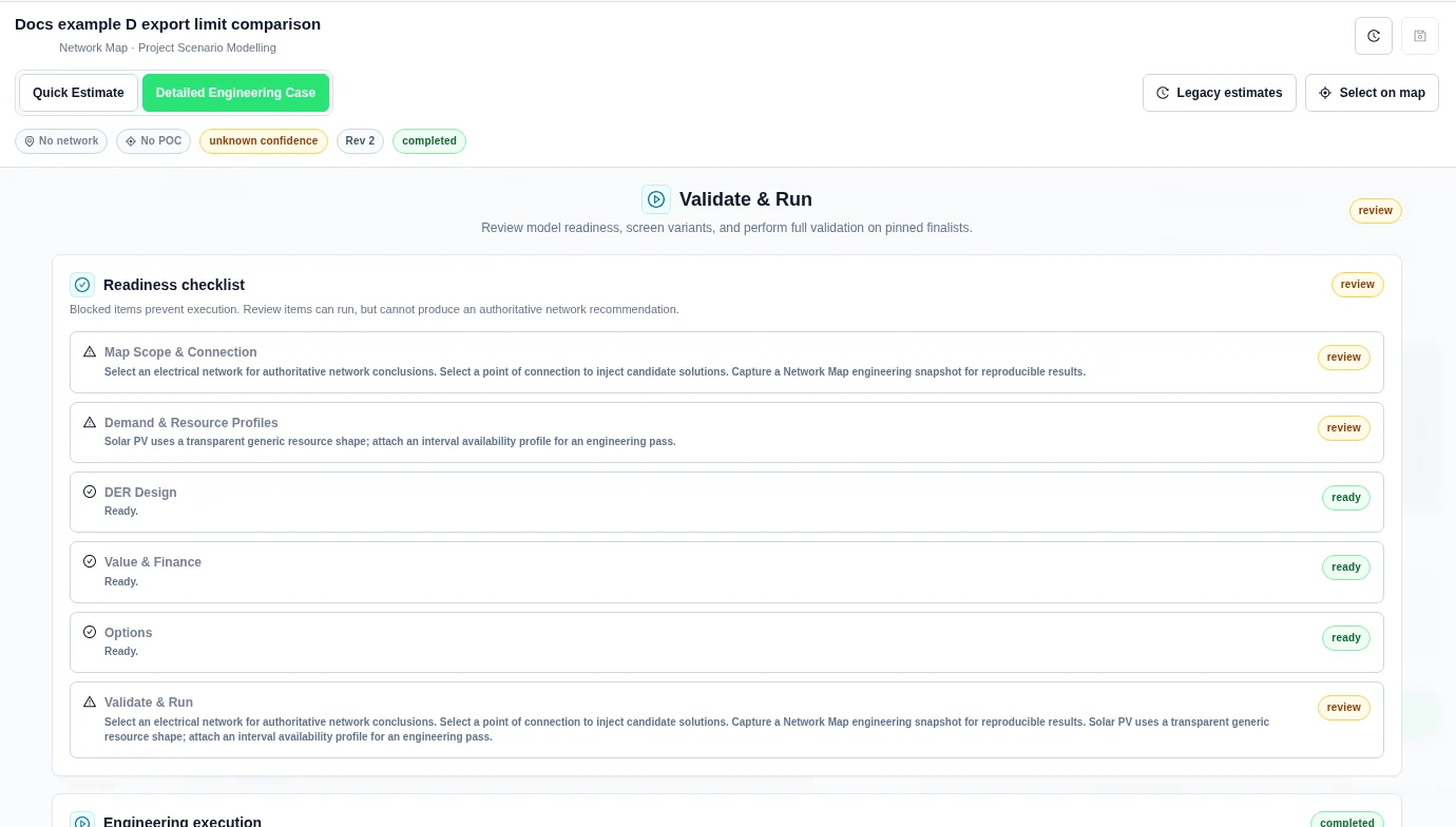
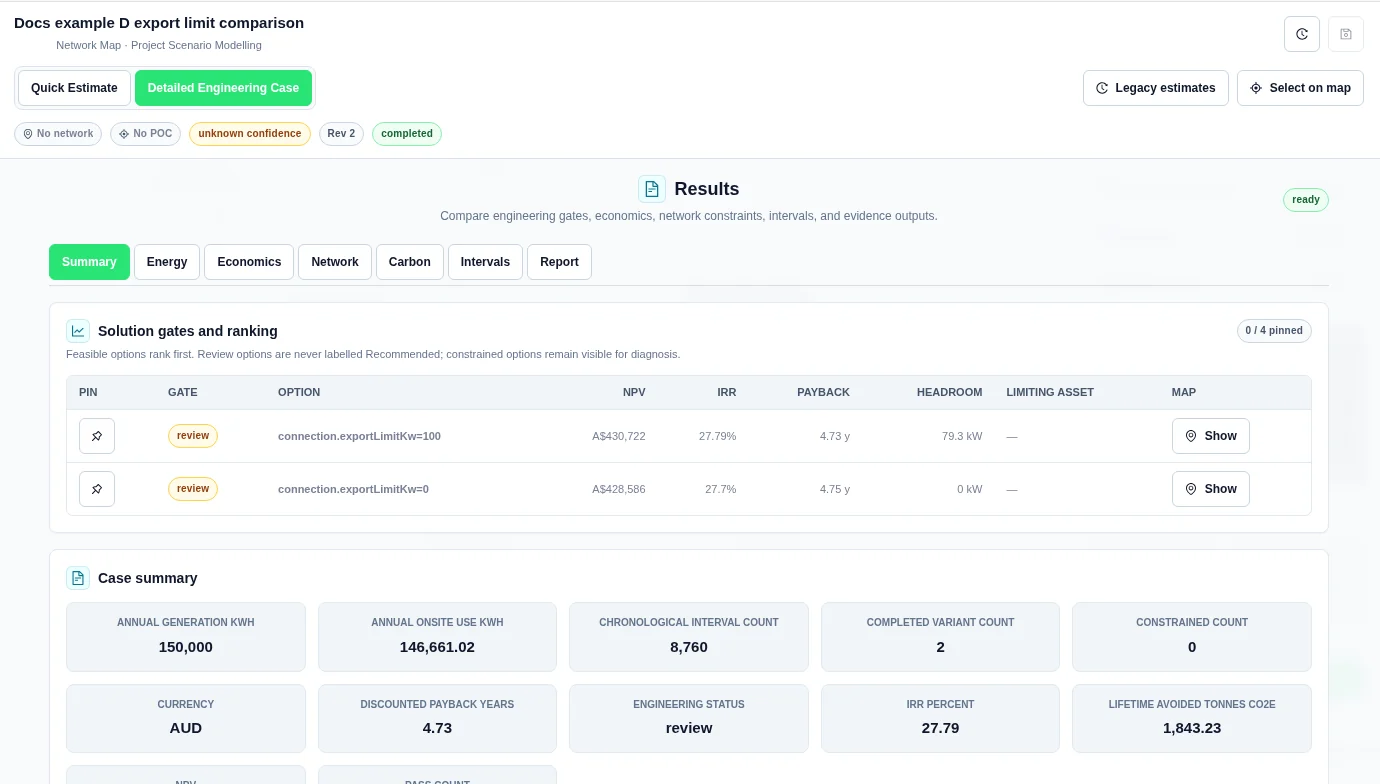
- After the run shows completed, open Results and read both rows in Solution gates and ranking.
Comparison as shown
| Option | Gate | NPV | IRR | Payback |
|---|---|---|---|---|
| connection.exportLimitKw=100 | review | A$430,722 | 27.79% | 4.73 y |
| connection.exportLimitKw=0 | review | A$428,586 | 27.7% | 4.75 y |
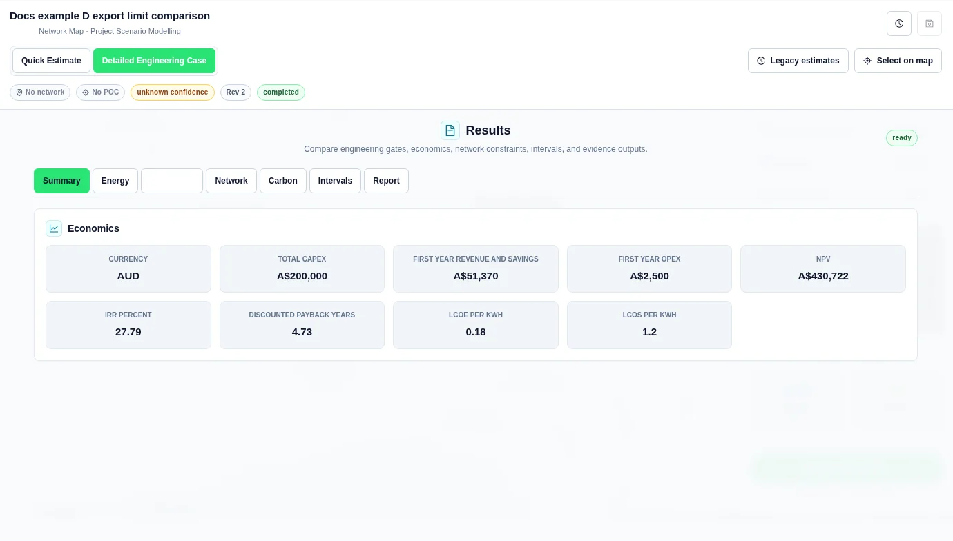
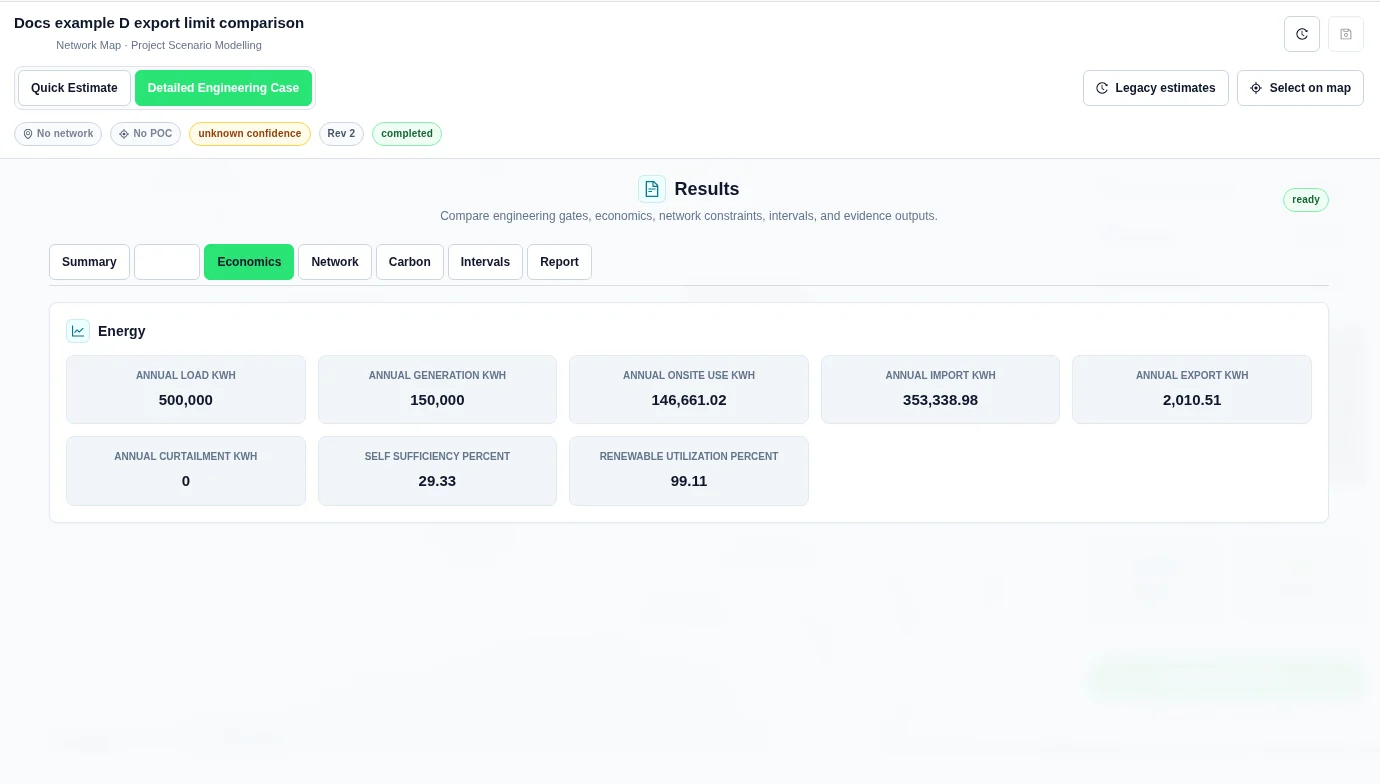
Leading option results as shown
The case summary and result cards show the leading 100 kW export-limit option.
| Input | Value |
|---|---|
| Total capex | A$200,000 |
| First year revenue and savings | A$51,370 |
| First year opex | A$2,500 |
| Annual generation | 150,000 kWh |
| Annual onsite use | 146,661.02 kWh |
| Annual import | 353,338.98 kWh |
| Annual export | 2,010.51 kWh |
| Annual curtailment | 0 kWh |
| Chronological interval count | 8,760 |
| Completed variant count / Pass count | 2 / 0 |
E. Riverbend cold store: compare nine solar and battery designs
Riverbend cold store is a fictional refrigeration site. Its cold rooms draw power overnight. Daytime handling and daily defrost cycles add to demand. Would a bigger rooftop array or a longer-duration battery repay its extra cost? This example holds the load and prices fixed and compares nine designs against buying all electricity from the grid.
Set up the comparison
- Use Detailed Engineering Case in Project Modelling. Give every option the same synthetic hourly load and solar profiles. The load is 595 MWh for the year, with a peak of 99.8 kW.
- In Design, pair one solar array with one AC-coupled battery. Keep battery power at 60 kW. Use size-based costs so the capital cost changes with the equipment size.
- In Options, sweep the solar generator’s modelled AC capacity over 120, 200, 280 kW and storage energy over 60, 120, 180 kWh. Each solar size is paired with each battery size, giving nine designs.
- Screen the nine variants, then open Results → Summary → Design value by solar size. Select a column to identify its equipment and read its NPV. Use the gates table to check what the screen assessed.
The results below come from these synthetic profiles. Substituting your site’s profiles or costs can change the order.
Inputs used for these results
- Profiles: 8,760 synthetic hourly values in 2025. The PV shape yields 1,453 kWh per kW of nameplate in the model year before curtailment. No customer meter or real site data was used.
- Operating limits: 150 kW import, 70 kW export. The battery serves onsite load, with 95% charge efficiency, 95% discharge efficiency and a 10–90% state-of-charge range.
- Value: 15 years at a 7% discount rate. Grid imports cost AUD 0.23/kWh and exports earn AUD 0.045/kWh. No inflation or price escalation; no revenue for demand reduction or backup operation.
- Equipment costs: solar AUD 1,150/kW; storage AUD 260/kW of power plus AUD 600/kWh of capacity. Annual operating costs are 1% of solar capex and 1.5% of storage capex. PV output degrades by 0.5% per year. The year 11 battery replacement allowance is 45% of battery capex.
Read the nine columns
The leftmost column has the highest net present value (NPV) among the designs tested. Colour identifies the solar PV nameplate (AC capacity in kW); it does not show battery size. Look for the same PV colour at different ranks to see how changing battery energy affected the result.
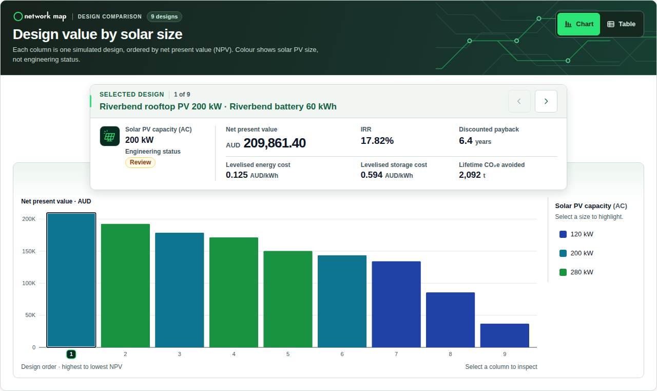
| Rank | Solar PV (kW) | Battery (kWh) | NPV (AUD) |
|---|---|---|---|
| 1 | 200 | 60 | 209,861 |
| 2 | 280 | 60 | 192,634 |
| 3 | 200 | 120 | 178,789 |
| 4 | 280 | 120 | 171,372 |
| 5 | 280 | 180 | 150,316 |
| 6 | 200 | 180 | 143,668 |
| 7 | 120 | 60 | 134,283 |
| 8 | 120 | 120 | 85,680 |
| 9 | 120 | 180 | 37,065 |
What changes at 280 kW?
Keep the 60 kW / 60 kWh battery and select the second column. The extra 80 kW of solar takes the upfront cost from A$281,600 to A$373,600. In the first year, exports rise from 35.1 to 102.8 MWh, while energy curtailed at the 70 kW export limit rises from 0.1 to 20.8 MWh. With exports worth 4.5¢/kWh against 23¢/kWh for avoided imports, the extra savings and export income do not cover the larger array’s additional costs over 15 years at the 7% discount rate.
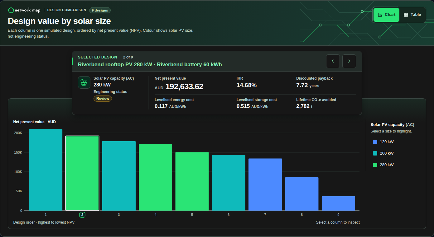
Limit: all nine designs have an engineering status of review. This is a chronological dispatch and financial screen with assumed limits, not an AC network study. No electrical network or connection rating was verified. The leading column is neither a connection approval nor a claim that this size is optimal. PV-only designs and other sizes were not tested.
How to read the design value chart · How NPV differs from annual cash flow.
Cash flow and reports
The versioned Economics tab shows metric cards and a separate Cashflow explorer. See Value and Finance for an annual table, CSV and reconciliation example. The Report view offers evidence and report controls.
Legacy Estimates has separate Cumulative Cash Flow and Annual Cash Flow charts. They belong to the legacy calculator, not the cases above. See the legacy guide before using that separate calculation path.
More tested examples
The following guides include more worked examples with explicit model assumptions:
- Shared Library: four-hour profile versions, a 2,000 AUD rate-card quote and a two-sheet workbook.
- Dispatch Calendars and Sizing: two solar sizes, with the fixed-cost warning retained.
- Asset Screening: genset fuel and costs, flexible-load capacity, fleet and on-demand charging.
- Contract Settlement: fixed price, CfD, swap and demand-response ledgers.
- Participant Allocation: a 60% share with 40% unassigned.
- Saved Reports and Templates: JSON export and a versioned DOCX template.
Related Guides
- Project Modelling
- Profiles and Inputs
- DER Design
- Value and Finance
- Network Tariffs
- Options and Results
- Comparison and Reports
- Legacy Estimates


