

Docs Menu
Options and Results
Generate design alternatives, validate their inputs, and interpret the resulting engineering evidence.
Watch the Video: Project Modelling: Getting Started (1:12)
Step 5: Create Options
Open Options. Quick Estimate calculates one design. Select Detailed Engineering Case to execute option sweeps.
- Choose Rank feasible solutions by.
- Review the initial Sweep 1, or select Add sweep.
- Choose Target asset.
- Choose Parameter.
- Enter the alternatives in Values, separated by commas.
- Check the variant count in Option generator.
A new case starts with a generator-capacity sweep of 250, 500, 750, 1000 kW. It uses Primary applicable asset. Select a named asset when several assets could match. Use the delete button on a sweep card to remove it. With no sweeps, the detailed case runs one design.
| Parameter | Target | Input |
|---|---|---|
| Generator capacity (kW) | Solar, wind, hydro, or biomass. | Installed generator capacity in kW. |
| Storage power (kW) | Battery storage. | Battery power rating in kW. |
| Storage energy (kWh) | Battery storage. | Battery energy capacity in kWh. |
| Storage reserve (%) | Battery storage. | Operating reserve percentage, consistent with the SOC window. |
| Export limit (kW) | The case connection, not an individual asset. | Compare alternative export limits in the model. |
Values must be finite, non-negative numbers. Repeated values count once. Check that a proposed size remains valid for the asset; the base design requires positive generation or storage capacity. Use one sweep per target field to keep the design intent clear.
Understand the variant limit
Sweeps form combinations. Three generator sizes and two storage sizes produce six variants. Adding four export limits produces 24 variants. The interactive limit is 250 variants. Reduce the number of values or remove sweeps if the counter exceeds 250.
Example: six battery alternatives
- Add one Battery storage asset with valid SOC limits and costs.
- Select Detailed Engineering Case and open Options.
- Remove the default generator sweep if it is not part of this comparison.
- Add a Storage energy (kWh) sweep with
100, 200, 400. - Add a Storage reserve (%) sweep with
10, 20. - Target the same battery in both sweeps. Check that the counter shows six variants.
- Screen the variants, review the evidence, and pin finalists.
This example shows how the combination count is calculated.
Choose a ranking metric
| Choice | Preferred direction |
|---|---|
| NPV | Higher. |
| IRR | Higher. |
| Discounted payback | Lower. |
| LCOE / LCOS | Lower. |
| Carbon reduction | Higher avoided emissions. |
| Connection headroom | Higher remaining connection capacity. |
NPV is the default. Engineering gates take precedence over the selected metric. A profitable constrained design is not made feasible by its financial result. See Comparison and Reports for financial comparison and sensitivity methods.
Step 6: Check readiness
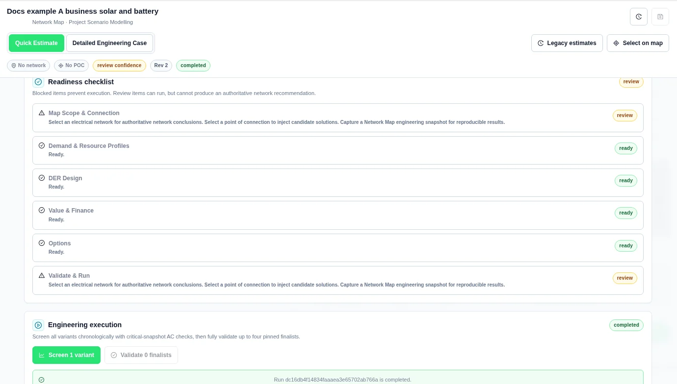
Open Validate & Run. Select a row in Readiness checklist to return to the relevant inputs.
| Status | Meaning |
|---|---|
| ready | The preflight checklist has no issue for that section. Run the assessment to review network results. |
| review | The case can run, but an input or assumption needs review before an authoritative network recommendation. |
| blocked | An input issue prevents execution. |
| pending | The required result is not available yet. |
Resolve blocking items
- Correct or detach invalid profiles.
- Add at least one DER or load-adjustment asset.
- Enter positive generator capacity, and positive storage power and energy.
- Make the battery SOC window valid.
- Give a load adjustment positive peak demand or annual energy.
- Use an analysis horizon greater than zero and a discount rate of zero or greater.
- Give each sweep valid values and a compatible target.
- Keep the option count at or below 250.
The service also validates the submitted specification. Correct any additional field error, including battery initial or terminal SOC outside the operating window, an invalid voltage band, or a profile interval mismatch.
Resolve review items
- Select an electrical network and point of connection.
- Capture the engineering snapshot.
- Attach a validated load profile for detailed work.
- Attach availability profiles for solar, wind, and hydro.
- Review the inverter and DC-bus assumptions for DC-coupled storage.
Screen and validate
- Check the intended case revision, inputs, and map snapshot.
- Select Screen. The button includes the number of variants.
- Wait for the run to complete and open Results.
- Review the gates and metrics in Summary.
- Pin up to four candidates with their Pin controls.
- Return to Validate & Run.
- Select Validate. The button includes the number of pinned finalists.
- Review the new result and the network evidence.
Detailed screening uses chronological dispatch and AC checks at selected critical snapshots. Finalist validation performs the broader AC assessment for the pinned options. Check the network evidence and diagnostics for the assessed intervals, limits and electrical inputs.
The case is saved as a revision before a run starts. The run ID appears in Engineering execution. Starting another run is disabled while the current run is submitting, queued, or running.
Run states and recovery
| State or control | Meaning and action |
|---|---|
| idle | No run has started in this workbench state. |
| submitting | The case and run request are being sent. Do not submit the same run again. |
| queued / running | Execution is waiting or active. Status refreshes automatically. |
| completed | Results are available. Read their engineering status separately. |
| failed | Read the error. Correct invalid inputs before starting a new run. |
| Cancel | Available while queued or running. It requests cancellation of the current run. |
| cancelled | The run was cancelled; it is not a completed engineering result. |
| Retry | Available after failure or cancellation when a run record exists. It retries that run specification. Use a new screen after changing case inputs. |
If The feasibility run service is not connected. or a start error appears, the run has not produced a result. If Run status could not be refreshed. appears, confirm the recorded run state before creating another run. A status-refresh error does not prove that the server calculation stopped.
Completed run with review items
Step 7: Read Summary
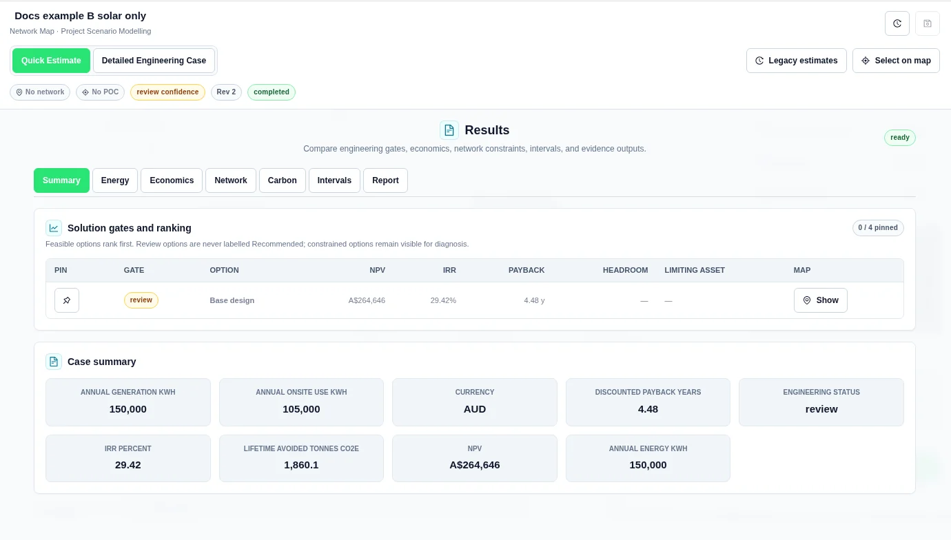
Solution gates and ranking lists all returned options.
| Column | Meaning |
|---|---|
| Pin | Select or remove a finalist. At most four options can be pinned. |
| Gate | Engineering status: pass, review, or constrained. |
| Option | The generated design name, with a recommendation marker to aid comparison. |
| NPV / IRR / Payback | Financial comparison metrics. Payback is discounted payback, in years. |
| Headroom | Remaining modelled connection capacity, in kW, when assessed. |
| Limiting asset | The asset identified by the network assessment, when available. |
| Map → Show | Display available result layers for that option. |
Interpret the engineering gate
- pass: the modelled checks support the case within the assessed scope.
- review: missing data, estimated inputs, or incomplete assessment prevents an authoritative conclusion.
- constrained: one or more assessed constraints are exceeded.
Pass options appear before review and constrained options. Review the limiting inputs before accepting any recommendation. Unknown values are unavailable, not zero. Missing unserved-energy, loading, violation-count, or network-coverage evidence cannot establish a pass. Do not treat a recommendation marker or table order as a substitute for these checks.
Case summary describes the selected aggregate result. The detailed result panels represent the selected result, not a separate full dashboard for every comparison row.
Read the design value chart
After screening the options, open Results → Summary → Design value by solar size. Each vertical column is one simulated design with a reported net present value (NPV). Read left to right from highest to lowest NPV. The horizontal axis is rank, not time. The vertical axis measures NPV in the case currency, not annual savings. A negative value extends below zero. An NPV of zero stays in the ranking; an unavailable NPV is not plotted.
Colour shows the total enabled solar PV nameplate capacity for that design, in kW. Add the AC capacity of the enabled Solar assets after the option’s size changes. This is not the array’s DC rating in kWp, the inverter limit, generated kWh or the battery size. Two columns of the same colour can represent different batteries. No solar (0 kW) is distinct from an unknown PV size.
Select a column to read its design, NPV, solar capacity and engineering status. Use Previous design and Next design to step through the options. With keyboard focus on the plot, use the left or right arrow, or Home and End. Solution gates and ranking groups options by engineering status and can order them differently. A high NPV is not an engineering pass.
Read all nine columns in the Riverbend cold store example.
Summary example
Energy, Network, and Carbon
| View | What to inspect |
|---|---|
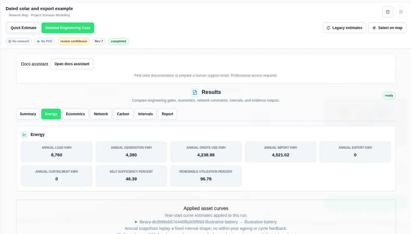
| Energy | Annual load, generation, onsite use, grid imports and exports, curtailment, self-sufficiency, and renewable utilization. Energy totals use kWh; ratios use percent. |
| Economics | Capital cost, first-year value and operating costs, NPV, IRR, payback, LCOE, and LCOS. Use Value and Finance for definitions and assumptions. |
| Network | Engineering status, connection headroom, limiting asset, and the assessment message. Check the evidence for evaluation coverage. Quick Estimate does not evaluate network constraints. |
| Carbon | First-year avoided emissions, lifetime avoided emissions, and first-year carbon value. Check the baseline emissions factor or profile used. |
Use Show result layers in Network when available. Layers can show modelled voltage and thermal loading for lines and transformers. Geometry, electrical inputs, and a calculated result must be available for an asset to appear. Missing map colour is not proof that an asset passed.
Intervals and charts
Open Intervals for Chronological interval results. The workbench shows at most 50 rows. Open Open Plot Studio for chart review. Check the source data and row counts before treating a preview as the complete annual series.
| Interval field group | Meaning |
|---|---|
| Timestamp and duration | The interval time and duration in hours. |
| Baseline load / load | Demand before and after the proposed load changes, in kW. |
| Generation / proposed generation / dispatchable generation | Total and component generation output, in kW. |
| Storage charge / discharge / SOC | Charging and discharging power in kW, and stored energy in kWh. |
| Import / export and baseline import / export | Grid exchange with and without the proposed design, in kW. |
| Baseline / scenario reactive power | Reactive power in kvar. |
| Curtailment | Generation that cannot be used or exported, in kW. |
| Unserved load | Demand not supplied in the interval, in kW. An unavailable value must not be read as zero. |
The returned chart set can include Chronological Dispatch (daily average), Validated Network Envelope, Annual Engineering Cash Flow, and Option Ranking — NPV for the default ranking metric. The daily-average dispatch chart shows load, generation, grid import/export, and storage charge/discharge. It does not show interval peaks. The network envelope shows minimum voltage, maximum voltage, and maximum thermal loading for the validated snapshots; these series have different units.
The detailed evidence can include Feasibility Option Comparison, Chronological Dispatch, Network Criteria, Critical Network Intervals, and Annual Cash Flow tables. The dispatch table can be truncated to 2,000 rows. The result evidence retains a compressed interval series. Check truncation and total-row metadata when extracting a full series; do not assume that a chart or table preview contains every interval.
Saved result lifecycle
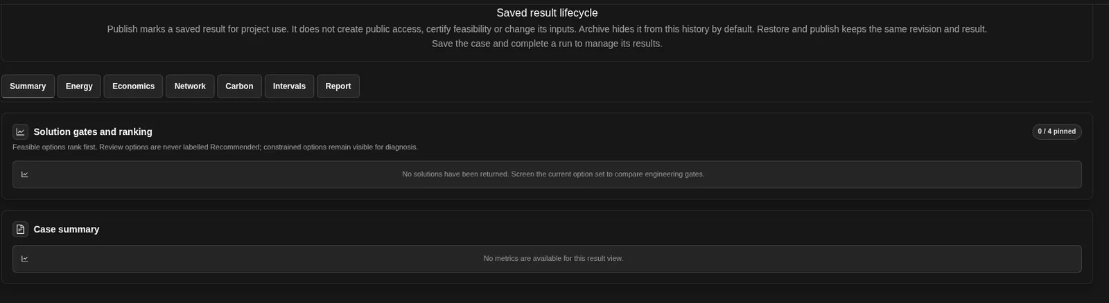
Under Results, Publication, evidence and sharing has a Saved result lifecycle part. Save the case and complete a run to manage its results:
- Publish marks a saved result for project use. Access permissions and saved inputs stay unchanged.
- Archive hides a result from this history by default.
- Restore and publish keeps the same revision and result.
Reports and follow-on studies
In Report, Engineering report pack provides Evidence ZIP, PDF summary, XLSX tables, CSV tables, and JSON manifest. Export presentation creates a separate presentation when a current eligible result exists. See Comparison and Reports for the formats and presentation procedure.
Continue engineering assessment offers Hosting Capacity, Connection Readiness, Contingency, Short Circuit, and Protection. Choose a follow-on study, confirm its scope and study-specific inputs, and run it separately.
Calendars, price experiments and bounded sizes
Options includes Dispatch calendars, a detailed-mode Dispatch price experiment, and Bounded financial sizing. Calendar bounds remain subject to scalar equipment and site limits. Decision-price experiments do not change settlement prices.
Bounded sizing compares at most 25 discrete candidates. This is separate from the option generator’s 250-variant limit above. It does not prove a global optimum. See Dispatch Calendars and Sizing for the tested two-size example and limitations.
Trace energy through the common bus
- Complete a Detailed Engineering Case and open Results → Energy.
- Under Aggregate energy path and balance, read the coverage statement before using totals.
- Use Previous interval and Next interval. Compare sources, targets and the residual for that interval.
The view is an accounting balance through a common bus. It is not a physical network diagram or a direct generator-to-consumer allocation. Unserved load is a reference, not an energy source. Storage charge and discharge are bus-side flows; internal storage losses are not added as another bus target.
Read identified asset paths
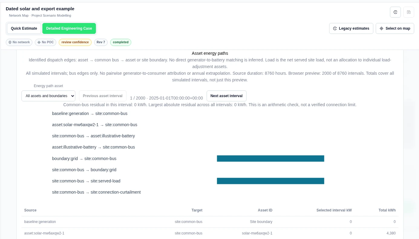
- Continue to Asset energy paths. Read its separate coverage statement.
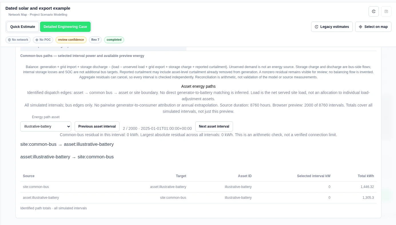
- Choose Energy path asset to focus on one equipment ID.
- Use Previous asset interval and Next asset interval. Compare selected-interval kW with Total kWh.
Worked example: solar and battery paths
Our synthetic 2 kW solar and 20 kW / 40 kWh battery run simulated 8,760 hourly intervals. The browser preview contained 2,000. The full identified-path totals showed solar to common bus 4,380 kWh, common bus to battery 1,446.32 kWh, battery to common bus 1,305.3 kWh, grid import 4,521.02 kWh and served load 8,760 kWh.
Match clean energy by hour
In Results, open Clean-energy matching for a saved Detailed run. Select Load saved-run source context. Set the Reporting timezone, Matching region, Eligible technologies and Policy source.
In Source ownership and qualification evidence, enter the source region, owner, retained attributes and supporting evidence. Set Require matching certificates to match your chosen policy. Use Policy permits attributes to follow stored energy when that policy allows source attributes to move through storage.

Choose Preview modelled matching to check the inputs. To keep an exact version, enter an Input version name, choose Save scope, and select Save inputs and analyse. Use Load pinned inputs and Replay pinned matching to reproduce that input version.
Worked example: solar, storage and hourly demand
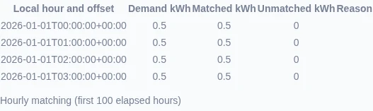
This saved four-hour example has 0.5 kWh of demand in each hour. Solar produces 1 kWh in each of the first two hours. The battery stores 0.5 kWh in each of those hours, then supplies 0.5 kWh in each of the final two hours. Its modelled charge and discharge efficiencies are both 100%.
The example matching policy retains solar ownership attributes through storage and does not require certificates. The modelled result for this example shows 2 kWh matched, an hourly matched-energy ratio of 100%, and 0 unknown hours. Each hour has 0.5 kWh matched demand and 0 kWh unmatched demand.
Expand Source conservation, storage pools and certificate balances to inspect where energy came from and how it passed through storage. Use Download interval ledger CSV for the flow ledger or Download matching evidence JSON for the complete result.
Related Guides
- Project Modelling
- Profiles and Inputs
- DER Design
- Value and Finance
- Comparison and Reports
- Engineering Plot Studio
- Running Engineering Studies
- Worked Examples


