

Docs Menu
Network Tariffs
Review tariff sources, author explicit rate rows, and keep screening assumptions separate from exact billing rules.
Browse published network tariff versions
Open Project Modelling → Value → Versioned retail and network tariffs. Set Tariff class to Network and select Load published versions. The catalogue loads 200 versions at a time. When the status says "More results are available.", select Load more published versions. This versioned catalogue is separate from the static network picker described later in this guide.
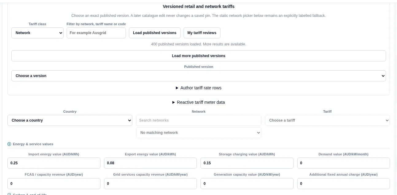
The catalogue now includes United States utility sources as well as Australia, Ireland, New Zealand and the United Kingdom. The network list is ordered by network name, so United States utilities appear first on the early pages.
Filter and select a source version
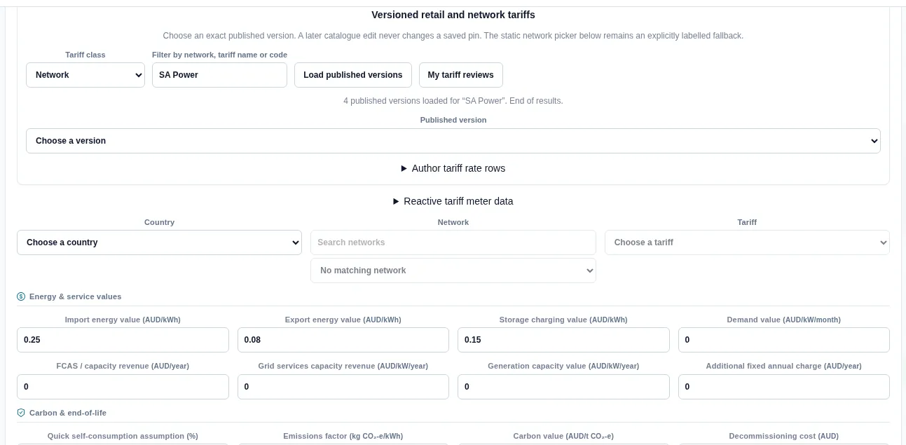
Enter a network, tariff name or code in Filter by network, tariff name or code, then select Load published versions. The filter searches the whole catalogue, not only the pages already loaded. "End of results." means every match is loaded. Choose a Published version. Read its version number, currency, timezone, effective dates and source.
Inspect rules before using rates
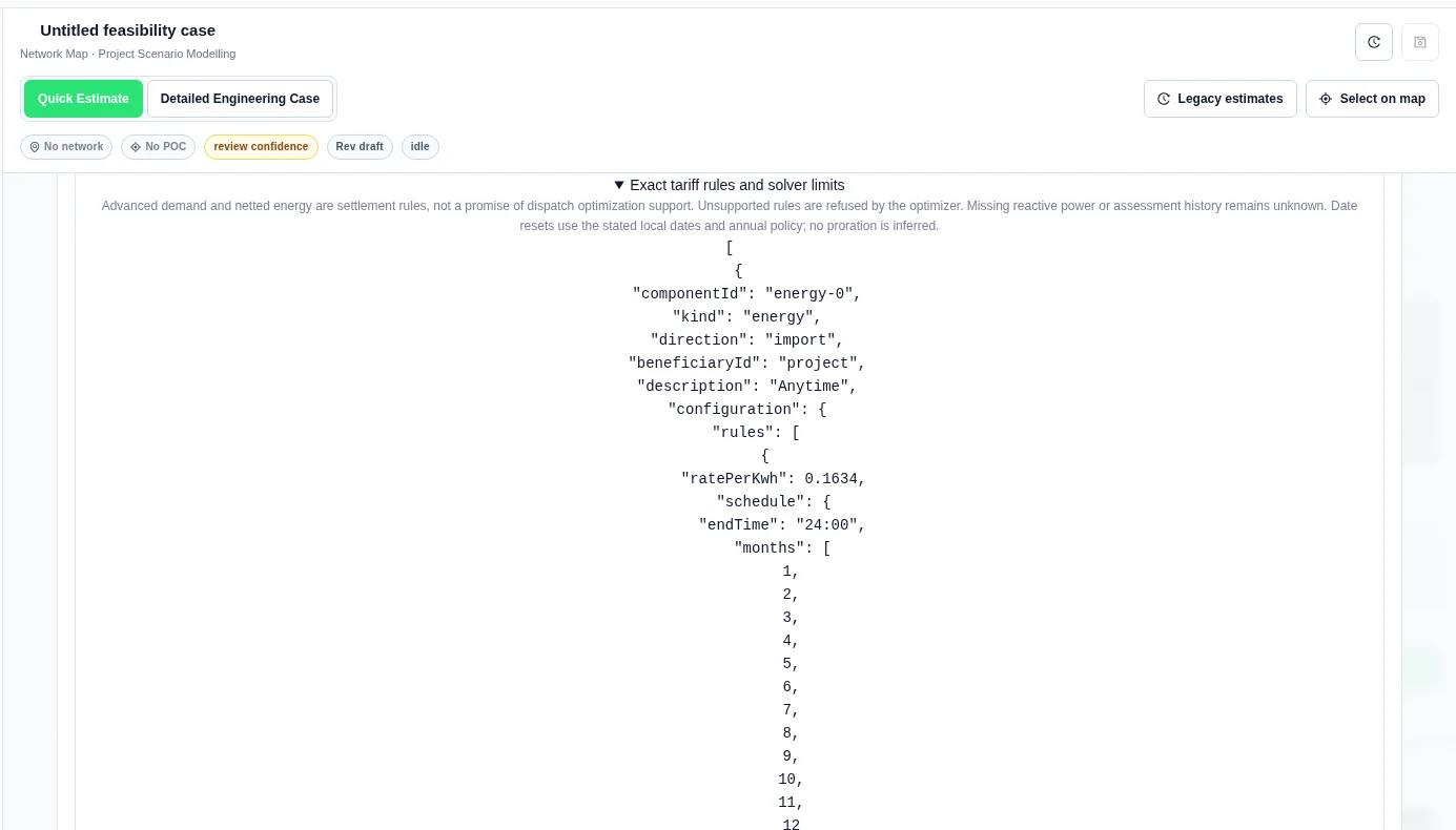
Expand Exact tariff rules and solver limits. Review each component, its schedule and the source qualifications. Check the original tariff document. Match currency, timezone, tariff dates, voltage, customer class and tax treatment to the study. Missing reactive power, demand history or qualifications remain unknown.
Worked example: review a published source
We selected Residential Single Rate · v1 · SA Power · 2026-07-01. The preview and rule details supplied:
| Field | Value shown |
|---|---|
| Currency and timezone | AUD; Australia/Adelaide |
| Effective dates | 1 July 2026–30 June 2027 |
| Anytime import energy rate | 0.1634 AUD/kWh |
| Fixed daily amount | 0.6815 AUD |
| Tax qualification | Source prices exclude GST |
| Source | SA Power Networks 2026–27 Customer Overview Document, Table 9 NUoS Tariff Schedule, cross-checked to the AER SCS pricing model |
This example reviews source metadata. The version retains its source-review qualification, and missing charges remain unavailable.
Author a private tariff version
- Open Value → Versioned retail and network tariffs → Author tariff rate rows.
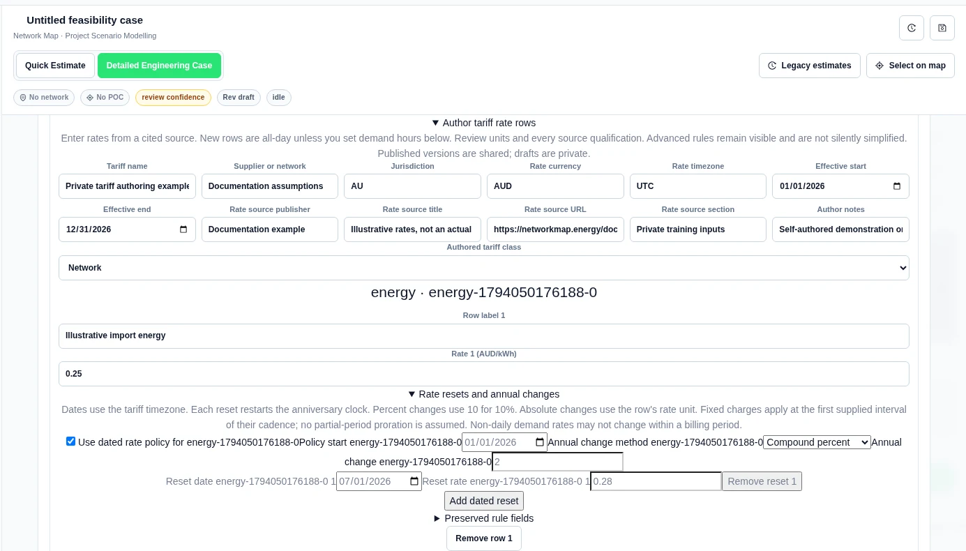
- Enter Tariff name, supplier, jurisdiction, currency, timezone, effective dates and source details. Use the source URL and section that support your rates.
- Select Add energy row, Add demand row or Add fixed row. Review each rate unit. New rows are all-day until the supported schedule fields are changed.
- Review Preserved rule fields. Copied advanced rules are kept, but not every rule has a visual editor.
- Confirm I checked all rates and qualifications in the source. Leave Share this published version clear to save a private draft. Select Save authored version.
A new version does not change old case pins. Record your source review and check the site qualifications for the selected tariff.
Add reactive meter data
- Under Versioned retail and network tariffs, expand Reactive tariff meter data.
- Prepare a CSV with the columns timestamp, baselineImportKvar, baselineExportKvar, projectImportKvar and projectExportKvar. Values are in kVAr.
- Select Upload reactive tariff CSV, then save the case.
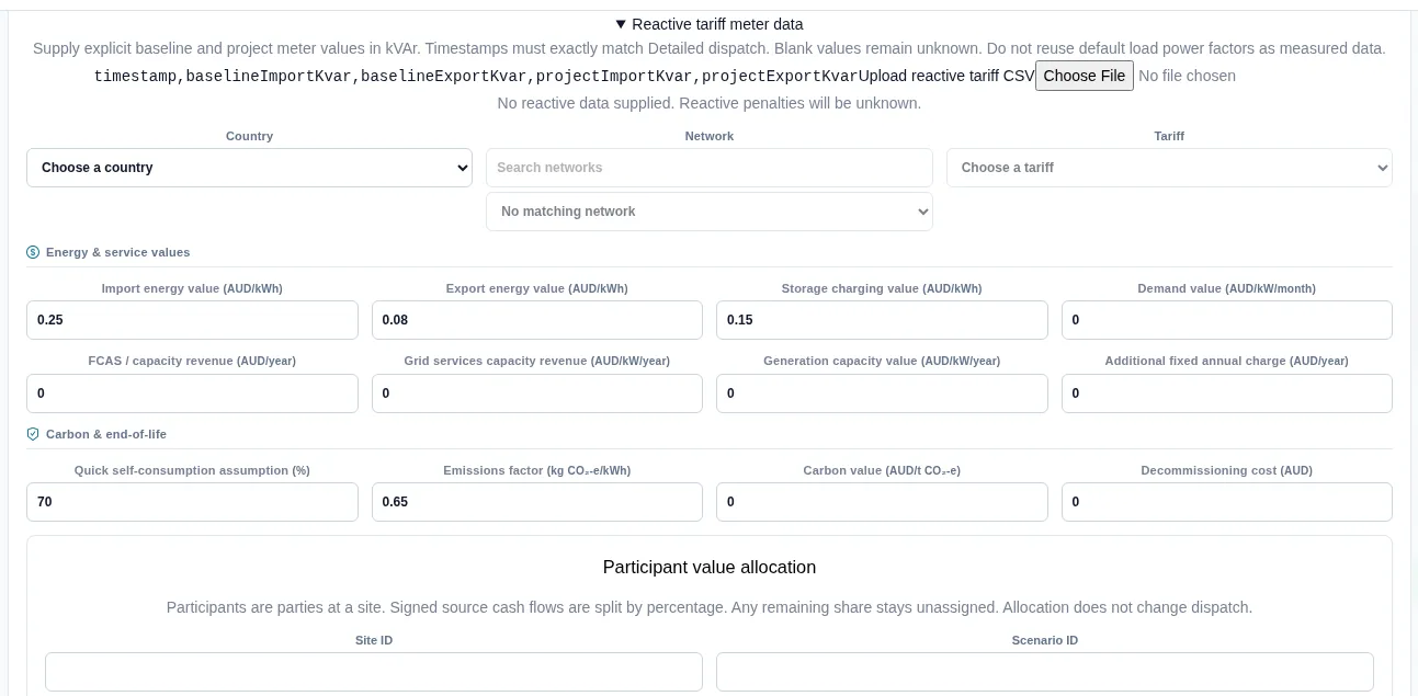
Timestamps must exactly match the Detailed dispatch intervals. Blank values stay unknown. Do not use a default load power factor as measured reactive data. Reactive data matters only for a tariff version that has kVAr or kVA rows.
Set dated rates and annual changes
- Expand Rate resets and annual changes for the row.
- Enable Use dated rate policy. Set Policy start, Annual change method and Annual change.
- Select Add dated reset for a known rate change. Enter its local date and rate.
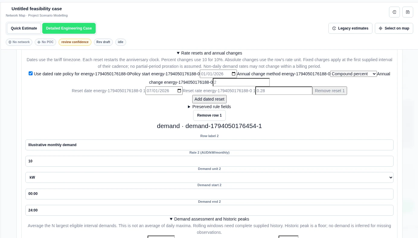
Compound percent, Linear percent and Absolute rate change have different meanings. Enter 10 for a ten-percent change. An absolute change uses the row’s rate unit. Non-daily demand rates cannot change within a billing period. No unsupported proration or recurring reset calendar is inferred.
Upload historic demand peaks
- Expand Demand assessment and historic peaks.
- Set Number of largest interval peaks and, if required by the source, Rolling assessment months and Minimum demand.
- Use Upload historic peak CSV. Its header is
date,demand,unit. Supply distinct dates, non-negative values and the exact demand-row unit. - Review Historic peak floor. Enter Historic peak expiry only when the source defines it.
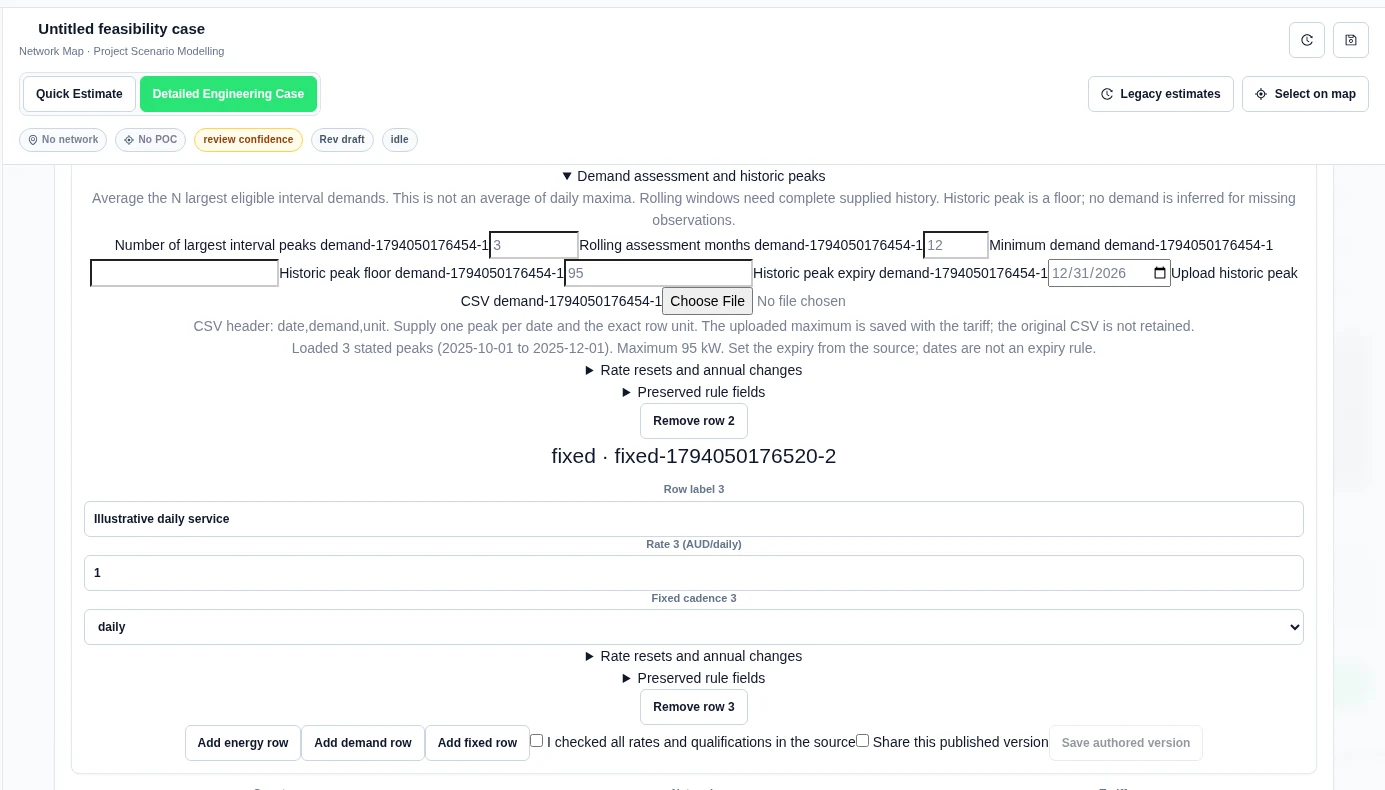
The average uses the largest eligible interval demands, not daily maxima. Rolling windows need complete history. The CSV limit is 1 MiB and 10,000 rows. The original file is not retained. No unit conversion, reactive-threshold penalty or missing demand is inferred.
Worked example: a private draft
We entered self-authored example rates. The form saved draft version 1 and reported Old pins are unchanged.
| Input | Value entered and retained |
|---|---|
| Currency and timezone | AUD; UTC |
| Effective dates | 1 January–31 December 2026 |
| Energy rate | 0.25 AUD/kWh |
| Demand rate | 10 AUD/kW/monthly |
| Fixed rate | 1 AUD/daily |
| Energy policy | 2% compound annual change from 1 January; reset to 0.28 AUD/kWh on 1 July 2026 |
| Demand assessment | 3 largest interval peaks; 12 assessment months |
| Historic CSV | 80, 95 and 90 kW on three distinct dates; uploaded maximum 95 kW |
This example covers rate authoring and intake. The example rates remain in a private draft.
What the static picker does
The Network tariff section is in Value & Finance. It uses a tariff library supplied with the application. It is separate from the network scope selection on the map.
The picker converts tariff components into an annual-average import energy value, a monthly demand value, and an annual fixed-charge assumption. It records the selected country, network, tariff, tariff year, and source. It does not reproduce a full retail bill.
Choose a static screening tariff
- Check the case Currency before choosing a tariff.
- In Country, select the tariff country.
- Use Search networks to filter by network name or state.
- Select the Network. The list shows the network name, state where supplied, and tariff count.
- Wait for the tariff file to load.
- Select a Tariff. Entries show their code and name where supplied.
- Read the tariff card and open Source when a source link is available.
- Check the preview values and any currency or coverage warning.
- Select Apply tariff.
- Review the updated values below the picker and save the case revision.
The picker can preselect a network that matches the case scope or previously applied tariff. You must still check the tariff selection. Changing country clears the network, tariff, and search. Changing network clears the tariff.
Countries, currencies, and customer classes
The supplied library includes the following country groups. Available networks and tariffs are listed in the picker.
| Country | Tariff currency |
|---|---|
| Australia | AUD |
| Ireland | EUR |
| New Zealand | NZD |
| United Kingdom | GBP |
| United States | USD |
Tariffs are grouped by customer class: Residential, Small business, Large business, High voltage, Subtransmission, Transmission, or Other. Available groups depend on the selected network.
If the tariff and case currencies differ, match the currency and review all case amounts before applying the rates. The picker does not perform foreign-exchange conversion.
Read the tariff card
| Card field | What to check |
|---|---|
| Tariff year | Published year or period. Not stated means the library does not provide it. |
| Structure | Flat, Time of use, Demand, Time of use + demand, or Capacity. Voltage is shown when supplied. |
| Fixed | Daily or annual fixed charge and its currency. |
| Energy | Each component rate in currency/kWh, with any day, hour, or month windows. |
| Demand | Each component rate in currency/kW/month, currency/kVA/month, or currency/kW/day. Check its demand basis and time window. |
| Tax | Includes GST/VAT, Excludes GST/VAT, or Not stated. This is source metadata, not a separate tax calculation. |
| Notes | Source conditions and qualifications, when provided. |
| Source | Link to the published source, when available. |
Missing metadata or an unpriced component is not proof of a zero charge. Check the source before using a missing value in a financial decision.
Ausgrid tariff example
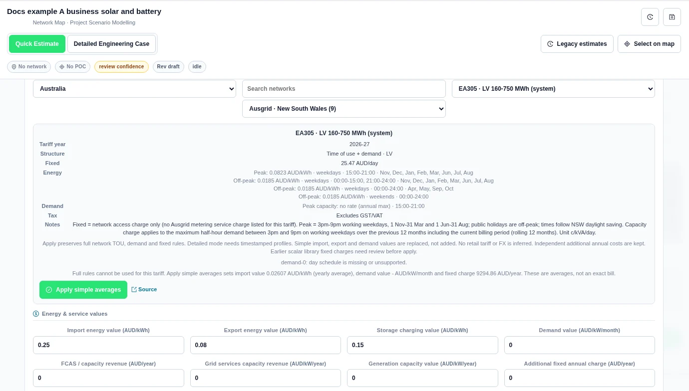
In example A, this sets the import value to 0.02607 AUD/kWh and the fixed annual charge to 9294.86 AUD. These cover network charges, not a complete retail bill. No library demand rate is available in this capture.
How the screening values are derived
Import energy value
The picker calculates a time-weighted average over the 2026 reference calendar. Each hour uses the matching rate. Where components overlap, the component covering fewer hours in the year takes priority. Hours without a matching rate are excluded.
This is an average by time, not an average weighted by your site's consumption. A partial-coverage message states how many hours are covered. Review that gap before using the average. The resulting Import energy value is rounded to five decimal places.
Demand value
The picker uses the first demand component with a usable rate. It does not add all displayed demand components together.
- A per-kW monthly rate is multiplied by the number of active months and divided by 12.
- For a valid baseline power factor greater than zero and no greater than one, a per-kVA monthly rate is divided by that power factor, then spread over 12 months in the same way.
- A per-kW daily rate is multiplied by the days in its active months and divided by 12.
Check the baseline power factor before applying a kVA tariff. The converted Demand value is in currency/kW/month and is rounded to four decimal places. This value is a simplified annualized assumption, not a replay of each demand-billing window.
Fixed annual charge
A daily charge is multiplied by 365. Otherwise, the stated annual charge is used. The Fixed annual charge is recorded to two decimal places.
What changes when you apply
- Only available derived values replace Import energy value, Demand value, and Fixed annual charge.
- A component without a usable rate leaves the existing corresponding value unchanged.
- Export energy value, storage values, asset costs, and other finance assumptions are not replaced.
- The Applied: indicator identifies the tariff and its year where available.
Applying a tariff copies a snapshot of values and source details. Review the values again when the tariff source changes. The case does not track a changing retailer contract automatically.
Loading and missing-data messages
| Message | Next step |
|---|---|
| Loading network tariffs. | Wait for the country and network lists. |
| Network tariffs are not available yet. Enter the rates below. | Enter verified rates manually in Value & Finance. |
| No matching network | Change the search text or country. |
| Loading tariffs | Wait before selecting a tariff. |
| Could not load tariffs for this network. | Select a different network, then return to the required network to retry. Alternatively, enter verified rates manually. |
| Currency mismatch | Use the same currency for tariff rates and the case. No automatic conversion is made. |
| Energy coverage warning | Check the uncovered hours and the source. Do not treat missing hours as free electricity. |
Retail export tariffs: private source review
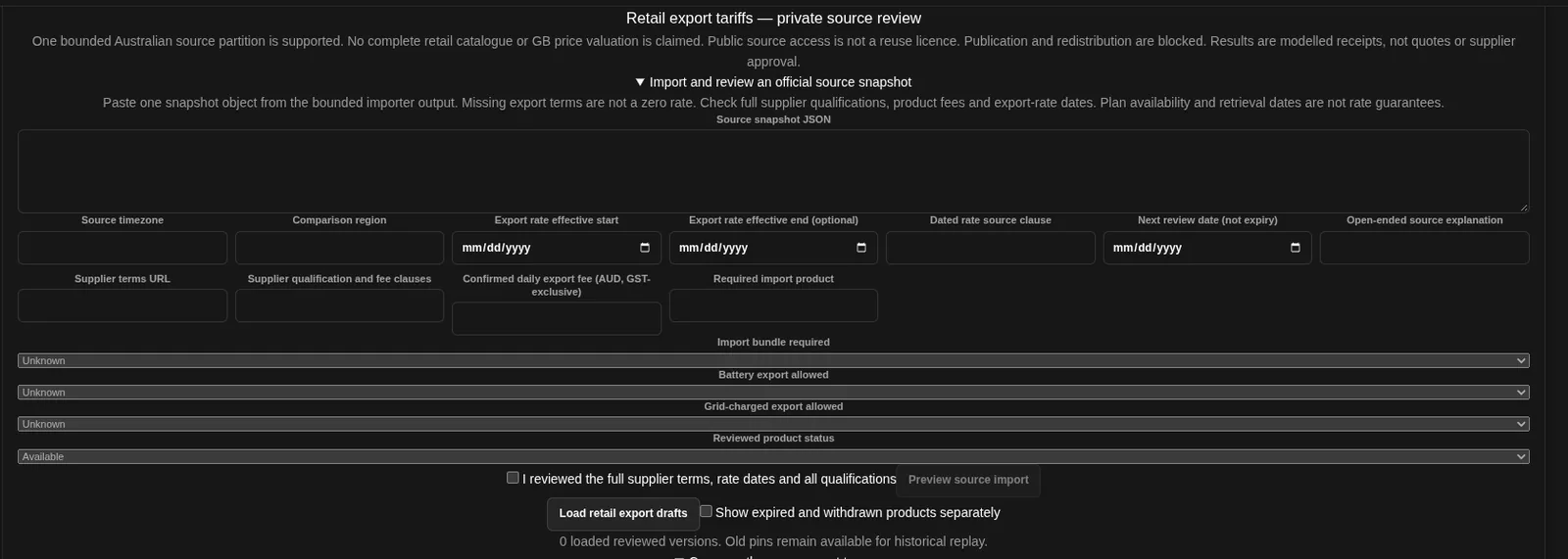
Find this in Value & Finance under Retail export tariffs — private source review. You paste one source snapshot from the importer and review it before it is used. The panel states its limits:
- One bounded Australian source partition is supported. No complete retail catalogue or GB price valuation is claimed.
- Public source access is not a reuse licence. Publication and redistribution are blocked.
- Results show modelled receipts using the reviewed source inputs.
- Missing export terms remain unavailable. Check the source-stated rate dates and terms before using a plan.
Fill in the source fields, such as the export rate start and end dates, the supplier terms URL and the daily export fee. Tick I reviewed the full supplier terms, rate dates and all qualifications, then choose Preview source import. Load retail export drafts loads the reviewed versions.
Compare assumptions with a retail bill
Use the source tariff and a bill to check your input assumptions. Keep energy rates, demand charges, and fixed charges separate. Confirm whether tax is included. Check the bill period and demand unit before converting a charge.
A network tariff can be only one part of a retail price. Do not add the same network charge twice when entering an all-in import value. Review the exported cash flows rather than treating the tariff preview as a bill total.
Legacy flat and time-of-use estimates
The legacy Tariff & Site Constraints section has a separate rate model. It uses manually entered flat or weighted rates, not the network tariff picker.
| Field | Default | Meaning |
|---|---|---|
| Tariff Model | Flat import rate | Choose a flat avoided import value or Time-of-use weighted rate. |
| Self-consumption (%) | 70% | Share of generation used onsite after curtailment. |
| Peak Rate | 0.30 per kWh | Peak energy value. |
| Peak Energy Share (%) | 35% | Weight of peak energy in the averaged import rate. |
| Shoulder Rate | 0.18 per kWh | Shoulder energy value. |
| Shoulder Energy Share (%) | 40% | Weight of shoulder energy. |
| Off-peak Rate | 0.10 per kWh | Off-peak energy value. |
| Off-peak Energy Share (%) | 25% | Weight of off-peak energy. |
| Demand Charge ($/kW-month) | 0 | Monthly rate used for demand savings. |
| Demand Reduction (kW) | 0 kW | Assumed reduction in billed demand. |
| Fixed Charge ($/day) | 0 | Daily charge deducted from legacy cash flows. |
| Curtailment (%) | 0% | Share of generation removed before onsite use and exports. |
Flat import rate uses Electricity Rate from Financial Assumptions. Time-of-use weighted rate uses:
Weighted rate = (peak rate × peak share + shoulder rate × shoulder share + off-peak rate × off-peak share) / total share.
Enter meaningful energy shares with a positive total. These are energy weights, not hourly schedules. The legacy model normalizes by their sum.
Legacy annual demand savings equal monthly demand charge × demand reduction × 12. The annual fixed cost equals the daily charge × 365. Both then use the legacy annual escalation multiplier.
With coordinated battery operation, time-of-use battery value uses the positive peak-minus-off-peak spread. Flat-rate operation uses the positive import-minus-export spread. This is a screening value, not chronological tariff dispatch.
Set source-stated demand windows
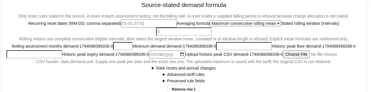
- In an authored demand row, expand Demand assessment and historic peaks → Source-stated demand formula.
- Enter Recurring reset dates (MM-DD, comma separated) only when the source states them. This restarts assessment history, not the billing rate.
- Choose Averaging formula. Supply the stated N or rolling window length. Do not infer a blank parameter.
- Review the source, interval coverage and refusal reasons before saving or settling.
| Averaging formula | Meaning |
|---|---|
| Existing interval peak rule | Keep the existing peak assessment. |
| Mean of all eligible intervals | Average every eligible supplied interval. |
| Mean of largest N intervals | Average the stated number of largest eligible interval demands, not daily maxima. |
| Maximum consecutive rolling mean | Form complete consecutive eligible windows, then select the largest mean. |
In the authoring example above, the editor retained two recurring dates and a window of 3 intervals. These example inputs were left unsaved. The published-source and historic-peak workflows are shown earlier in this guide.
Optimise bounded demand rules
- Set the demand row's Averaging formula and its parameters from your source.
- In Options, enable Use joint optimisation in Detailed Analysis.
- Save and run the Detailed Engineering Case. In Results → Report, download the JSON manifest and inspect joint-dispatch-objective.

Worked example: a four-hour demand bill
The example uses a 0, 3, 0 and 1 kW load across four one-hour UTC intervals. Storage was 1 kW / 2 kWh, with 50% opening and terminal SOC and 100% charge and discharge efficiency. The grid import limit was 3 kW and export was 0 kW.
| Example demand rule | Saved method | Exact settlement |
|---|---|---|
| Maximum two-interval rolling mean, 20 AUD/kW | joint_convex_lp | 20 AUD |
| Decreasing blocks: 8 AUD/kW to 0.5 kW, 2 AUD/kW to 1.5 kW, then 1 AUD/kW | joint_bounded_milp | 6.5 AUD |
Both saved results returned optimal. Solver cost and exact settlement reconciled with a 0 AUD difference. These are interval bills for the supplied four-hour examples. See Dispatch Calendars and Sizing for the workflow.
Related Guides
- Project Modelling
- Value and Finance
- Profiles and Inputs
- Comparison and Reports
- Unit Revenue with Loss Factors
- Worked Examples


