Market analysis of 17 November 2026
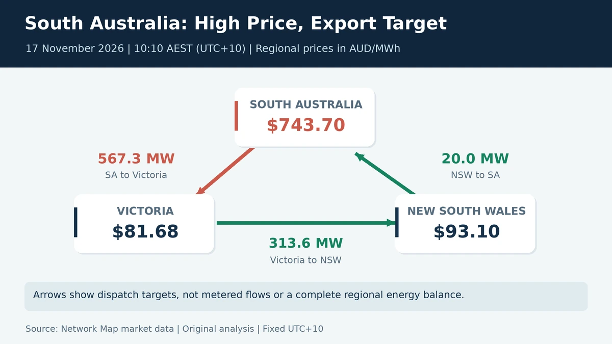
A high regional electricity price does not guarantee an import target on every connecting line. At 10:10 on 17 November, South Australia’s price was $743.70/MWh while the Heywood interconnector had a 567.3 MW target towards Victoria, where the price was $81.68/MWh.
That is a counter-price target: the scheduled direction runs from the higher-priced region to the lower-priced region. Across the seven-day sample, these targets occurred in 64.2% of matched New South Wales-South Australia records, 42.6% for Heywood and 21.3% for Victoria-New South Wales. The analysis below uses dispatch targets, not meter readings, and joins prices at the same published timestamp.
Start With The Same Five Minutes
At the same 10:10 timestamp, New South Wales was priced at $93.10/MWh. The New South Wales to South Australia interface, associated with EnergyConnect, had a 20.0 MW target towards South Australia. The Victoria to New South Wales interface had a 313.6 MW target towards New South Wales.
The three selected targets therefore formed a directional loop: South Australia to Victoria, Victoria to New South Wales, and New South Wales to South Australia. This is not a complete regional energy balance. Other interconnectors, generation, demand and network losses are outside that three-arrow picture.
Targets Are Not Meter Readings
The official market-data definition distinguishes the target for the next five minutes from metered telemetry. For the 10:10 EnergyConnect record, the target was 20.0 MW towards South Australia, but the metered field was approximately 5.9 MW in the opposite direction. Heywood’s metered field was approximately 577.2 MW towards Victoria, compared with its 567.3 MW target.
These are different fields: a dispatch target and a SCADA flow value, not two interchangeable measurements. A shared record timestamp does not establish simultaneous target and metered conditions. Mixing a target on one interface with a metered value on another can create a misleading picture. The comparison below consistently uses dispatch targets, with prices joined to the same published five-minute timestamp.
Count The Pattern, Not Just One Snapshot
We matched 2,016 timestamps across three regional price series and three interconnector series, from 17:25 on 10 November to 17:25 on 17 November. One expected timestamp, 16:10 on 13 November, was absent across these series. It was not interpolated or counted.
An interval was counted as counter-price when its signed target pointed from the higher-priced region to the lower-priced region. Both flow directions were tested. Equal prices and zero targets were not counter-price cases, but remained in the denominator.
- New South Wales-South Australia: 1,294 of 2,016 matched timestamps, or 64.2%.
- Heywood: 858 of 2,016, or 42.6%.
- Victoria-New South Wales: 429 of 2,016, or 21.3%.
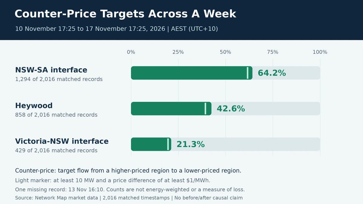
As an analyst-chosen sensitivity check, we required |target| ≥ 10 MW and |price difference| ≥ $1/MWh. Using the same denominator, the counts became 1,243, 793 and 395. These thresholds exclude small-magnitude observations; they are not an industry materiality standard.
What The Count Does Not Prove
These unweighted shares describe only 10–17 November. They do not establish a post-commissioning trend, a causal price effect, traded energy, trading profit or loss-adjusted settlement residues. A trend test would need defined comparison periods and controls for changing network conditions.
The official explanation of transmission-loop settlement arrangements provides the wider context. Dispatch accounts for the connected network, losses and operating constraints. A counter-price direction on one part of a loop is not, on its own, proof of network malfunction.
Why It Matters For Market Studies
For a project study, the useful question is not simply whether a line imports or exports. It is which flow field is being used, which prices it is paired with, and what network limits applied at that time. Those distinctions matter when connecting price exposure, connection constraints and revenue assumptions.
Our 9 November South Australia analysis examined an earlier price spike and counter-price exports. This newer comparison adds a matched multi-interval view rather than treating another single snapshot as a trend.
Sources And Method
WattClarity’s 17 November report provided the topic prompt. Network Map independently joined regional energy prices to interconnector records for the timestamp-level analysis.
The source records are AEMO-derived seven-day Network Map market-data snapshots retrieved at 17:26 on 17 November. The price endpoint reports RRP in AUD/MWh. Each interconnector series contains both MWFLOW, the target for the next five minutes, and METEREDMWFLOW, the SCADA value. Only MWFLOW is used in the counter-price calculation. All times are interval-ending, fixed UTC+10.
Source directions come from the public AEMO INTERCONNECTOR table: NSW1-SA1 maps NSW1 to SA1, V-SA (Heywood) maps VIC1 to SA1 and VIC1-NSW1 maps VIC1 to NSW1. AEMO’s dispatch definition says positive flow starts at REGIONFROM.
The inclusive seven-day endpoints contain 2,017 expected five-minute timestamps. The 2,016 matched timestamps omit 16:10 on 13 November, which was absent across the analysed series. No value was interpolated.
For each interface, the test is MWFLOW × (destination price − source price) < 0. Both flow directions are included. Zero targets and equal prices are not counter-price cases and remain in the denominator. Each timestamp has equal weight.
Download the matched records and verification script. The bundle contains the exact four market snapshots, matched-interval CSV, direction records, method notes and a standard-library Python verification script.
Use the live-market guide to add regional price and interconnector context, then use the constraints workflow for limits and notices. The downloadable comparison is an independent timestamp analysis, not a native counter-price classification in the Network Map interface.